Experiment description
Opportunistic potatoes are a pest that affect farms in many negative ways and need to be controlled. This experiment attempts to find the economically optimal dose of a specific treatment for this purpose.
In the original experiment 8 measures were taken for various cultivars and doses, but we will restrict ourselves to only two now.
Introduction and disclaimer
The data collected pertains to a specific set of conditions, and we should not try to extend the results beyond that setting without seriously considering and accounting for any systematic differences between that setting and any broader setting.
The data analysed here is inherently random. If the data collection were to be repeated then the results will differ. We will try to estimate the extent to which this will be the case, but those estimates are themselves uncertain.
While the computer software used is tried and tested, the analysis involves multiple human elements. Both the client and statistician may have introduced human error at various stages of the research process.
Thus, no guarantee can ultimately be given on the correctness of any findings below.
Links are given occasionally to sources explaining the statistical concepts addressed. These are colloquial sources to aid understanding, not reference sources. However, most of these sources link to reference sources should the researcher require academic references for specific topics.
options(scipen = 90)
library(openxlsx)
library(plyr)
library(knitr)
library(viridisLite)
filecore <- 'Potatoes'
rawdata <- read.xlsx(paste0(filecore,'.xlsx'),'Export')
metadata <- read.xlsx(paste0(filecore,'.xlsx'),'Metadata')
Mapping <- read.xlsx(paste0(filecore,'.xlsx'),'Mapping')
alpha <- 0.05Basic data properties
The significance level chosen is 0.05. This means that we only look at results where the p-value is less than 0.05, as other results could easily just be chance variation.
rawdata$Cultivar <- unlist(mapvalues(rawdata$Cult, Mapping[1,4:(3+Mapping$NumLevels[1])], Mapping[1,9:(8+Mapping$NumLevels[1])]))
rawdata$Herbicide <- unlist(mapvalues(rawdata$Treat, Mapping[2,4:(3+Mapping$NumLevels[2])], Mapping[2,9:(8+Mapping$NumLevels[2])]))
Cultivars <- unlist(Mapping[1,9:(8+Mapping$NumLevels[1])])
nCult <- length(Cultivars)
Herbicides <- unlist(Mapping[2,9:(8+Mapping$NumLevels[2])])
nTreat <- length(Herbicides)
MeasureCols <- 4:5
Xmat <- rawdata[,MeasureCols]
Xbin <- (Xmat>0)+0
nMeasures <- ncol(Xmat)
MeasureNames <- names(Xmat)
MeasureNamesLong <- metadata$Description[MeasureCols]
nTotal <- nrow(Xmat)We separate out the factors that are presumed to cause differences in response (Cultivar and Herbicide) from the measurable outcomes that are presumed to be affected by the factors (TuberNumber, TuberMass).
Multivariate analysis
When tests are done on multiple factors or multiple outcomes then it increases the false positive rate. We normally allow a small posibility for false positives in order to maintain a reasonable power to detect true positives; but repeated testing increases this rate to the point were false positives are virtually guaranteed, which is not acceptable. Two approaches are used to combat this problem.
The first and best is to do a global test of general significance. The second is we adjust the probabilities to account for the fact that we are doing multiple tests. According to the Holm-Bonferroni method we compare the smallest p-value to \(\alpha\)/(number of tests)=0.0125, the second smallest to \(\alpha\)/(number of tests - 1), and so on.
As a starting point, we convert each explanatory variable into a binary (zero-one) variable based on whether it has a value of zero or larger than zero. Then we can calculate the average rate of response for each treatment within cultivar, and overall.
pvals_multi1 <- rep(NA,nCult)
tbl.rel <- tbl.abs <- vector('list',nCult)
for (i in 1:nCult) {
  cat('\n\n---\n\nOverall response to treatment for cultivar',Cultivars[i],'where 0 is no tubers and 1 is at least some tubers.\n\n')
  cultpos <- rawdata$Cultivar==Cultivars[i]
  cultdata <- Xbin[cultpos,]
  tbl.rel[[i]] <- round(apply(cultdata,2,function(x) { unlist(tapply(x,rawdata$Herbicide[cultpos],mean,na.rm=TRUE)) } ),2)
  print(kable(t(tbl.rel[[i]])))
  tbl.abs[[i]] <- apply(cultdata,2,function(x) { unlist(tapply(x,rawdata$Herbicide[cultpos],sum,na.rm=TRUE)) } )
  # pvals_multi1[i] <- chisq.test(tbl.abs, simulate.p.value = TRUE)$p.value
  # cat('\n\nWith the p-value being',round(pvals_multi1[i],3),'\n\n')
}
Overall response to treatment for cultivar Cultivar1 where 0 is no tubers and 1 is at least some tubers.
| Control | T0.20x | T0.40x | T0.60x | T0.80x | |
|---|---|---|---|---|---|
| TuberNumber | 1 | 0.25 | 0 | 0 | 0 |
| TuberMass | 1 | 0.25 | 0 | 0 | 0 |
Overall response to treatment for cultivar Cultivar2 where 0 is no tubers and 1 is at least some tubers.
| Control | T0.20x | T0.40x | T0.60x | T0.80x | |
|---|---|---|---|---|---|
| TuberNumber | 1 | 0 | 0.25 | 0.25 | 0 |
| TuberMass | 1 | 0 | 0.25 | 0.25 | 0 |
Overall response to treatment for cultivar Cultivar3 where 0 is no tubers and 1 is at least some tubers.
| Control | T0.20x | T0.40x | T0.60x | T0.80x | |
|---|---|---|---|---|---|
| TuberNumber | 1 | 0.25 | 0 | 0.25 | 0 |
| TuberMass | 1 | 0.25 | 0 | 0.25 | 0 |
Overall response to treatment for cultivar Cultivar4 where 0 is no tubers and 1 is at least some tubers.
| Control | T0.20x | T0.40x | T0.60x | T0.80x | |
|---|---|---|---|---|---|
| TuberNumber | 0.75 | 0.5 | 0 | 0 | 0.25 |
| TuberMass | 0.75 | 0.5 | 0 | 0 | 0.25 |
cat('\n\n---\n\nOverall response to treatment for all cultivars where 0 is no tubers and 1 is at least some tubers.\n\n')Overall response to treatment for all cultivars where 0 is no tubers and 1 is at least some tubers.
tbl.rel.allCult <- round(apply(Xbin,2,function(x) { unlist(tapply(x,rawdata$Herbicide,mean,na.rm=TRUE)) } ),2)
print(kable(t(tbl.rel.allCult)))| Control | T0.20x | T0.40x | T0.60x | T0.80x | |
|---|---|---|---|---|---|
| TuberNumber | 0.94 | 0.25 | 0.06 | 0.12 | 0.06 |
| TuberMass | 0.94 | 0.25 | 0.06 | 0.12 | 0.06 |
Due to the extreme dependence between the measurements, we cannot tests the measurements jointly for interaction with the treatment.
We consider the measurements one at a time, remembering that many are directly dependent on each other.
Univariate testing
In cases where a variable is numeric we often use Analysis of Variance (ANOVA) to check whether there is a difference in numeric response between groups.
However, the ANOVA assumes that the unexplained variation follows a bell-shaped density pattern. This assumption does not hold at all for this data, inflating the probability of a false positive result greatly. Sometimes the shape can be corrected using a power transformation but not in this case.
An alternative is a non-parametric procedure such as the Kruskal-Wallis approach. It is similar in principle, but safer (though less powerful).
We also do \(\chi^2\) (Chi Square) tests for each binary response. We make the assumption that the expected number of responses in every treatment is the same for a single variable. We then calculate the probability of seeing differences in the categories as large or larger that what we observe under the assumption. If this probability is small we conclude that there is evidence of differences.
StatsBasic <- c('Mean','SD','Median','LowerQ','UpperQ','Min','Max')
nStatsBasic <- length(StatsBasic)
nCult1 <- nCult+1
StatsArray<- array(9999.9, c(nStatsBasic, (nCult+1), nMeasures, nTreat))
for (i in 1:(nCult1)) {
  if (i > nCult) { cultpos <- 1:nTotal } else { cultpos <- rawdata$Cultivar==Cultivars[i] }
  cultdata <- Xmat[cultpos,]
  x <- rawdata$Herbicide[cultpos]
  for (j in 1:nMeasures) {
    y <- cultdata[,j]
    StatsArray[1,i,j,] <- unlist(tapply(y,x,mean,na.rm=TRUE))
    StatsArray[2,i,j,] <- unlist(tapply(y,x,sd,na.rm=TRUE))
    StatsArray[3,i,j,] <- unlist(tapply(y,x,median,na.rm=TRUE))
    StatsArray[4,i,j,] <- unlist(tapply(y,x,quantile,0.25,na.rm=TRUE))
    StatsArray[5,i,j,] <- unlist(tapply(y,x,quantile,0.75,na.rm=TRUE))
    StatsArray[6,i,j,] <- unlist(tapply(y,x,min,na.rm=TRUE))
    StatsArray[7,i,j,] <- unlist(tapply(y,x,max,na.rm=TRUE))
  }
}
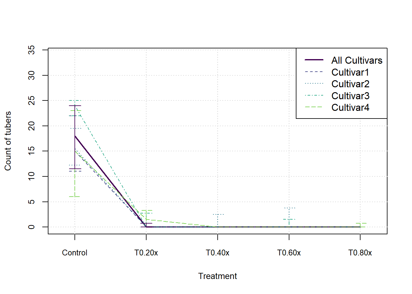
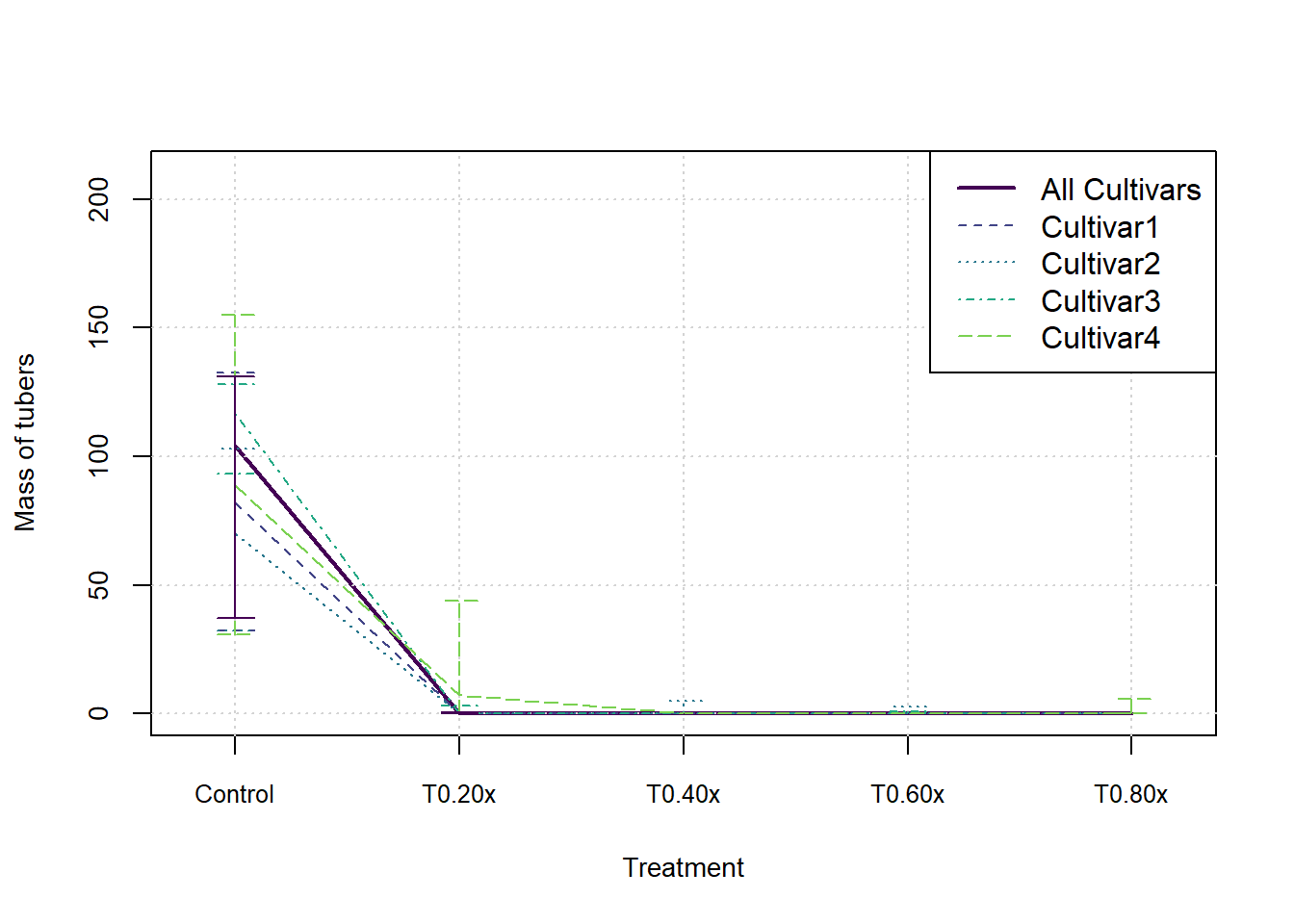
In the following graphs we show the median and inter-quartile range for each measure, split by cultivar. These do not indicate an statistical significance, they merely summarise the patterns in the data visually.
cols <- viridis(nCult+2)
xax <- 1:nTreat
for (j in 1:nMeasures) {
  plot(xax, StatsArray[3,nCult1,j,], type = 'l', col=cols[1], lwd=2, xlim = c(0.8,nTreat+0.2), ylim = c(0,max(StatsArray[7,nCult1,j,])), xaxt='n', xlab = 'Treatment', ylab=MeasureNamesLong[j], cex.lab= 0.88, cex.axis=0.88)
  axis(side = 1, at=xax, labels = Herbicides, cex.axis=0.8)
  grid()
  for (i in 1:nCult) {
    lines(xax, StatsArray[3,i,j,], col=cols[i+1], lwd=1, lty=(i+1))
    arrows(x0=xax, y0=StatsArray[4,i,j,], x1=xax, y1=StatsArray[5,i,j,], length=0.1, angle=90, code=3, col = cols[i+1], lwd=1, lty = (i+1))
  }
  arrows(x0=xax, y0=StatsArray[4,nCult1,j,], x1=xax, y1=StatsArray[5,nCult1,j,], length=0.1, angle=90, code=3, col = cols[1], lwd=1)
  legend('topright',c('All Cultivars',Cultivars), lwd=c(2,rep(1,nCult)), lty=1:nCult1, col=cols[1:nCult1])
}
Test results
TestNames <- c('KWpval','ANOVApval','ChiSQpval','Shapiro')
nTests <- length(TestNames)
nCult1 <- nCult+1
TestResults <- vector('list',nTests)
names(TestResults) <- TestNames
AllCultivars <- c(Cultivars,'All Cultivars')
for (k in 1:nTests) {
  TestResults[[k]] <- matrix(9.9,nCult1,nMeasures)
  rownames(TestResults[[k]]) <- AllCultivars
  colnames(TestResults[[k]]) <- MeasureNames
}
for (i in 1:(nCult1)) {
  if (i > nCult) { cultpos <- 1:nTotal } else { cultpos <- rawdata$Cultivar==Cultivars[i] }
  cultdata <- Xmat[cultpos,]
  x <- rawdata$Herbicide[cultpos]
  for (j in 1:nMeasures) {
    y <- cultdata[,j]
    TestResults$KWpval[i,j] <- kruskal.test(y,x)$p.value
    currlm <- lm(y~x)
    TestResults$ANOVApval[i,j] <- anova(currlm)$'Pr(>F'[1]
    Obs <- unlist(tapply(Xbin[cultpos,j],x,sum,na.rm=TRUE))
    Expec <- rep(mean(Obs),length(Obs))
    TestResults$ChiSQpval[i,j] <- 1-pchisq((2*sum(Obs*log(Obs/Expec))), nTreat-1)
    TestResults$Shapiro[i,j] <- shapiro.test(residuals(currlm))$p.value
  }
}
# TestResults
Based on the results of the Shapiro-Wilk test for Normality below and a visual analysis of the data, it is clear that an ANOVA is not appropriate for this data as its assumptions are markedly violated.
Shapiro-Wilk p-values:
result <- t(round(TestResults$Shapiro, 4))
kable(result)| Cultivar1 | Cultivar2 | Cultivar3 | Cultivar4 | All Cultivars | |
|---|---|---|---|---|---|
| TuberNumber | 0 | 0.0038 | 0.0254 | 0.0009 | 0 |
| TuberMass | 0 | 0.0009 | 0.0000 | 0.0072 | 0 |
Instead we consider the results of the Kruskal-Wallis tests and note that many p-values are small enough to reject the assumption of no difference in location between treatments. This implies that the treatment does have an effect on the measurements obtained.
Kruskal-Wallis p-values:
result <- t(round(TestResults$KWpval, 4))
kable(result)| Cultivar1 | Cultivar2 | Cultivar3 | Cultivar4 | All Cultivars | |
|---|---|---|---|---|---|
| TuberNumber | 0.0025 | 0.0124 | 0.0056 | 0.0578 | 0 |
| TuberMass | 0.0025 | 0.0078 | 0.0056 | 0.0699 | 0 |
The above is corroborated by the \(\chi^2\) tests, although those can only be done on all the cultivars grouped together.
Chi-square p-values:
result <- round(TestResults$ChiSQpval[nCult1,], 4)
kable(result)| x | |
|---|---|
| TuberNumber | 0.0001 |
| TuberMass | 0.0001 |
Lastly, we give the ANOVA results for interest.
ANOVA p-values:
result <- t(round(TestResults$ANOVApval, 4))
kable(result)| Cultivar1 | Cultivar2 | Cultivar3 | Cultivar4 | All Cultivars | |
|---|---|---|---|---|---|
| TuberNumber | 0.0005 | 0.0014 | 0 | 0.0113 | 0 |
| TuberMass | 0.0015 | 0.0020 | 0 | 0.0761 | 0 |
NB: An ANOVA or related test only tests whether an effect might be present, it does not explain what that effect might be. To investigate the effect further we must do additional testing.
Pairwise testing
A common approach to investigating the differences between means is Tukey’s HSD test. However, the assumptions of this test do not hold for our data, so we will use a non-parametric equivalent. It is known as the pairwise Wilcoxon or Mann-Whitney test.
The results are not significant for any one cultivar on its own, so only the tables for the cultivars as a group are given below.
Pairwise comparisons using Wilcoxon rank sum test
x <- rawdata$Herbicide
for (j in 1:nMeasures) {
  y <- Xmat[,j]
  cat('\n\nFor measurement:',MeasureNamesLong[j],'\n\n')
  print(kable(pairwise.wilcox.test(y,x)$p.value))
  cat('\n\n---\n\n')
}
For measurement: Count of tubers
| Control | T0.20x | T0.40x | T0.60x | |
|---|---|---|---|---|
| T0.20x | 0.0000547 | NA | NA | NA |
| T0.40x | 0.0000238 | 0.8982193 | NA | NA |
| T0.60x | 0.0000498 | 1.0000000 | 1 | NA |
| T0.80x | 0.0000161 | 0.8622252 | 1 | 1 |
For measurement: Mass of tubers
| Control | T0.20x | T0.40x | T0.60x | |
|---|---|---|---|---|
| T0.20x | 0.00027 | NA | NA | NA |
| T0.40x | 0.00002 | 1 | NA | NA |
| T0.60x | 0.00002 | 1 | 1 | NA |
| T0.80x | 0.00002 | 1 | 1 | 1 |
We see in the tables above that the 80% treatment and sometimes the 60% treatment are better than the 20% treatment. However, we see no evidence in the data that treatment at 80% or 60% is better than 40%. It may well be the case that higher treatments would show improved results if the experiment were expanded but this cannot be established in either direction via the above methods.
Regression analysis
The goal here is to determine whether there is some ideal level of treatment, based on the measurements taken. This is not a simple task as any simple model will not address the research question. Instead we fit a model that more closely resembles the true nature of the data. The current gold standard for implementing such complex models is the STAN interface. We will attempt to use this interface via RSTAN to implement our models.
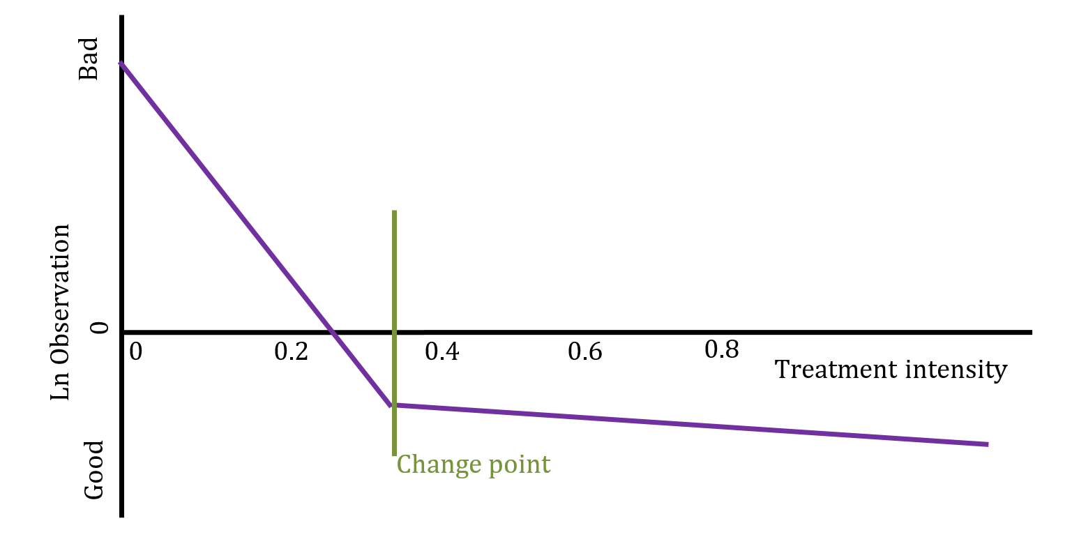
For this analysis, assume that the treatment increases in effectiveness as the dose is increased, but only up to a point, from which a higher dose no longer adds value to the enterprise. To test this we fit a model with two slopes and an unknown change point, then test whether the slopes fit our assumption. If the slopes do meet our expectations then we report the estimated change point as a proposed optimal treatment level.
This type of model is called a bi-phasic regression. Given an unknown changepoint \(\gamma\), the model is formally defined as \(y_i\sim N(\beta_0+\beta_1(x_i-\gamma)I(x_i>\gamma)+\beta_2(x_i-\gamma)I(x_i<\gamma),\ \sigma^2)\).
However, as noted previously, the observed data does not follow a Normal distribution. To bring the data in line with this assumption we make adjustments. First, we take the log of the observations. Since we can’t take the log of zero, we must treat them separately. The zeros do not occur randomly, they carry valuable information that must be incorporated into the model.
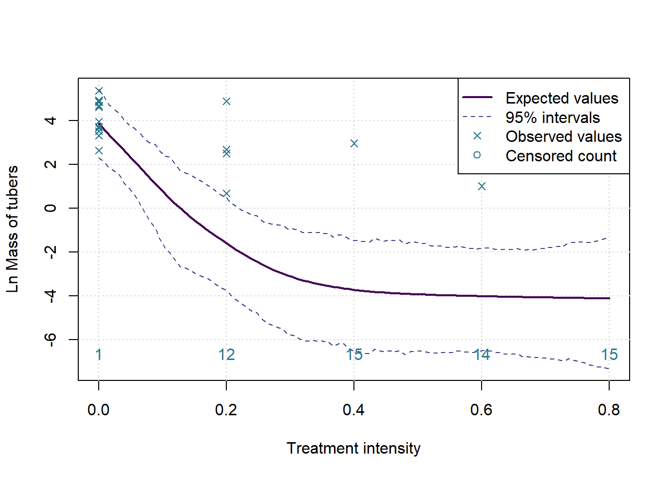
The approach implemented here is to consider zeros as values censored below a lower measurement limit. In the real experiment tubers cannot occur in non-whole numbers, but if it was possible then it would be reasonable to assume that the data generating process would want to produce numbers that are close to but not exactly zero, and certainly less than one. We assume that, based on a level of treatment, the experiment should have produced a real number of tubers greater than zero and less than one in all the cases where we observe a zero. On a log scale this implies a negative number of log tubers.
The proposed model is illustrated below:
 ```
```
suppressPackageStartupMessages(library(rstan,warn.conflicts=FALSE,quietly=TRUE))
options(mc.cores = 3)
rstan_options(auto_write = TRUE)
data {
int<lower=0> nobs;
vector[nobs] xobs;
vector[nobs] yobs;
int<lower=0> ncen;
vector[ncen] xcen;
real<upper=0> cen;
}
parameters {
real<upper=cen> ycen[ncen];
real<lower=0.1,upper=0.7> cp;
real b0;
real b1;
real b2;
real sigma;
}
model {
cp ~ uniform(0.1,0.7);
for (i in 1:nobs)
yobs[i] ~ normal(b0 + b1 * (xobs[i] - cp) * (xobs[i] > cp) + b2 * (xobs[i] - cp) * (xobs[i] < cp), sigma);
for (j in 1:ncen)
ycen[j] ~ normal(b0 + b1 * (xcen[j] - cp) * (xcen[j] > cp) + b2 * (xcen[j] - cp) * (xcen[j] < cp), sigma);
}
s_posterior <- vector('list',nMeasures)
for (k in 1:nMeasures) {
  yallfull <- Xmat[,k]
  ymiss <- is.na(yallfull)
  yall <- yallfull[!ymiss]
  xx <- rawdata$TreatIntensity[!ymiss]
  censored <- (yall<=0)
  yobs <- log(yall[!censored])
  xobs <- xx[!censored]
  xcen <- xx[censored]
  cen <- 0
  nobs <- sum(!censored)
  ncen <- sum(censored)

  s_data <- list(yobs=yobs, xobs=xobs, xcen=xcen, cen=cen, nobs=nobs, ncen=ncen)

  s_run<-sampling(splitreg, s_data, pars=c("b0", "b1","b2","cp","sigma"), chains=3, iter=4000, algorithm='HMC')
  s_post <- extract(s_run)
  s_posterior[[k]] <- s_post
}

saveRDS(s_posterior, "stanoutput.Rds")
pvalfunc <- function(sims,target=0) { 2*min(mean(sims<target),mean(sims>target)) }
hpd.interval <- function(postsims,alpha=0.05) { # Coded by Sean van der Merwe, UFS
sorted.postsims <- sort(postsims)
nsims <- length(postsims)
numints <- floor(nsims*alpha)
gap <- round(nsims*(1-alpha))
widths <- sorted.postsims[(1+gap):(numints+gap)] - sorted.postsims[1:numints]
HPD <- sorted.postsims[c(which.min(widths),(which.min(widths) + gap))]
return(HPD) }
for (k in 1:nMeasures) {
s_post <- s_posterior[[k]]
cat('\n\nConsidering measure:',MeasureNamesLong[k],'\n\n')
pval <- pvalfunc(s_post$b1+s_post$b2)
reject <- (pval<alpha)
pvalflat <- pvalfunc(s_post$b1)
accept <- (pvalflat>alpha)
cat('The p-value for the changepoint test is:', round(pval,4), 'and for the test of a flat slope after the changepoint the p-value is:', round(pvalflat,4), '\n\n')
cp_int <- hpd.interval(s_post$cp, alpha)
if (reject && accept) {
cat('Which means we assume there is a changepoint, with expected value ',round(mean(s_post$cp),2)*100,'% of recommended treatment, and 95% HPD interval of ',round(cp_int[1],2)*100,'% to ',round(cp_int[2],2)*100,'%.\n\n---\n\n',sep = '')
} else {
cat('Which means there is not enough evidence in the data to suggest a changepoint followed by a flat slope.\n\n---\n\n')
}
}Considering measure: Count of tubers
The p-value for the changepoint test is: 0.0047 and for the test of a flat slope after the changepoint the p-value is: 0.6583
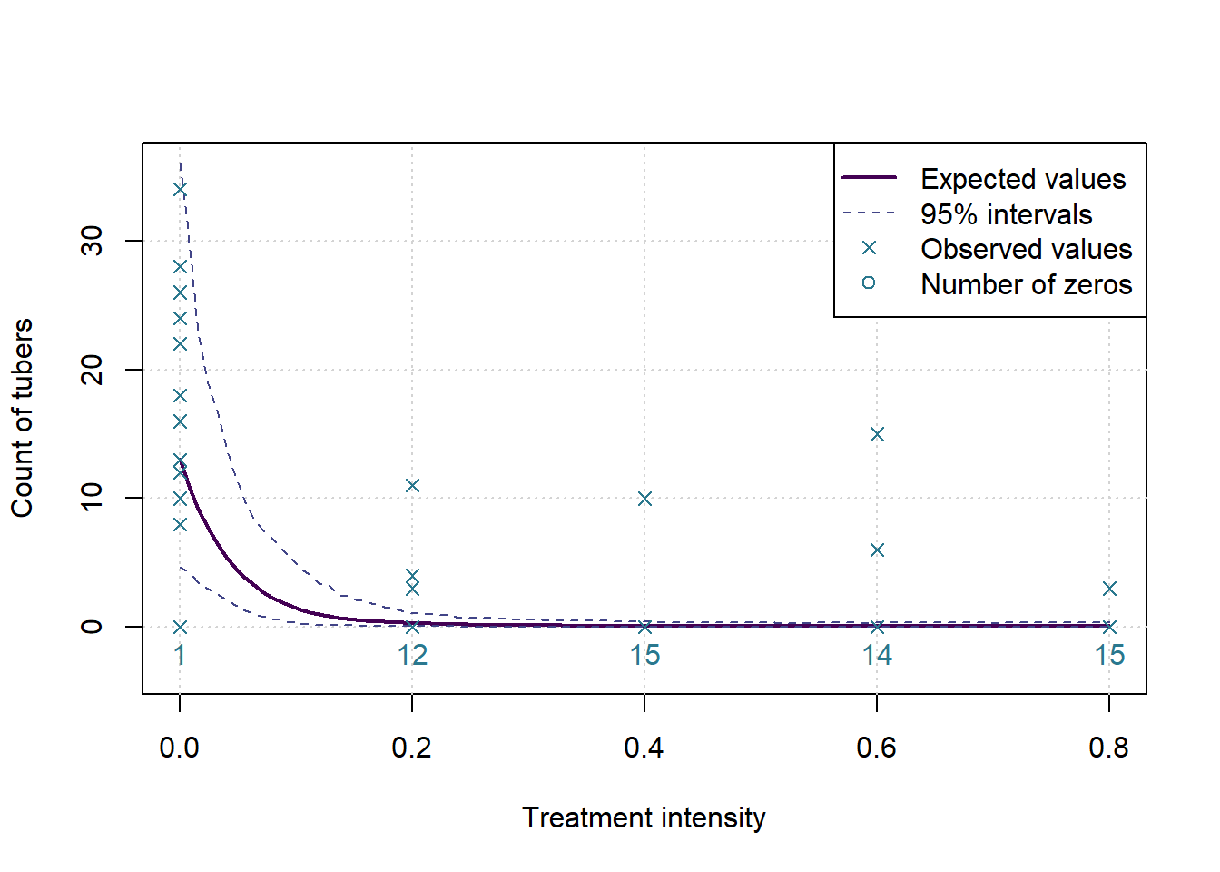
Which means we assume there is a changepoint, with expected value 24% of recommended treatment, and 95% HPD interval of 10% to 42%.
Considering measure: Mass of tubers
The p-value for the changepoint test is: 0.0087 and for the test of a flat slope after the changepoint the p-value is: 0.7993
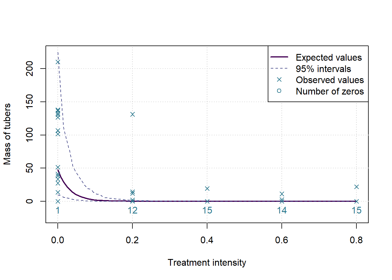
Which means we assume there is a changepoint, with expected value 27% of recommended treatment, and 95% HPD interval of 10% to 46%.
acc <- 101
grphx <- seq(0,0.8,length.out = acc)

for (k in 1:nMeasures) {
  sp <- s_posterior[[k]]
  sims <- sapply(grphx, function(x) { sp$b0 + sp$b1 * (x - sp$cp) * (x > sp$cp) + sp$b2 * (x - sp$cp) * (x < sp$cp) } )
  ints <- apply(sims,2,hpd.interval,alpha)

  yallfull <- Xmat[,k]
  ymiss <- is.na(yallfull)
  yall <- yallfull[!ymiss]
  xx <- rawdata$TreatIntensity[!ymiss]
  numzeros <- tapply(yall,xx,function(x){ sum(x==0) })

  ymax <- max(max(exp(ints[2,])),max(yall))
  plot(c(0,0.8),c(-0.1*ymax,ymax),type='n', ylab=MeasureNamesLong[k], main='', xlab='Treatment intensity')
  grid()
  lines(grphx,exp(colMeans(sims)), col=cols[1], lwd=2, lty=1)
  lines(grphx,exp(ints[1,]), col=cols[2], lwd=1, lty=2)
  lines(grphx,exp(ints[2,]), col=cols[2], lwd=1, lty=2)
  points(xx,yall, col=cols[3], pch=4)
  text(as.numeric(names(numzeros)), 0, labels = numzeros, pos = 1, col = cols[3])
  legend('topright',legend = c('Expected values','95% intervals','Observed values','Number of zeros'), lwd = c(2,1,NA,NA), lty=c(1,2,NA,NA), pch = c(NA,NA,4,1), col= cols[c(1,2,3,3)])

  ymax <- max(max(ints[2,]),max(log(yall),na.rm = TRUE))
  ymin <- min(-0.1*ymax,min(ints[1,]))
  plot(c(0,0.8),c(ymin,ymax),type='n', ylab=paste('Ln',MeasureNamesLong[k]), main='', xlab='Treatment intensity')
  grid()
  lines(grphx,colMeans(sims), col=cols[1], lwd=2, lty=1)
  lines(grphx,ints[1,], col=cols[2], lwd=1, lty=2)
  lines(grphx,ints[2,], col=cols[2], lwd=1, lty=2)
  points(xx,log(yall), col=cols[3], pch=4)
  text(as.numeric(names(numzeros)), ymin, labels = numzeros, pos = 3, col = cols[3])
  legend('topright',legend = c('Expected values','95% intervals','Observed values','Censored count'), lwd = c(2,1,NA,NA), lty=c(1,2,NA,NA), pch = c(NA,NA,4,1), col= cols[c(1,2,3,3)])

}