Case study: The Challenger data

Introduction

We proceed with a logistic regression analysis of the famous Challenger O-ring data, but from a Bayesian perspective.

Data and properties

The data is available here.

alpha <- 0.1 # The chosen significance level for intervals
library(openxlsx)
alldata <- read.xlsx('challenger.xlsx','Challenger')
n <- nrow(alldata)

The significance level chosen is 0.1. This means that we only look at results where the p-value is less than 0.1, as other results could easily just be chance variation.

The current gold standard for implementing advanced Bayesian models is the STAN interface. We will attempt to use this interface via RSTAN to implement our models.

suppressPackageStartupMessages(library(rstan,warn.conflicts=FALSE,quietly=TRUE))
options(mc.cores = 3)
rstan_options(auto_write = TRUE)

The logistic regression model

We first define the model.

//
// This Stan program defines a basic logistic regression with a single predictor.
// The code below is by Sean van der Merwe, UFS
//
// The input data is a vector 'y', its length 'n', and its explanatory predictor 'x'.
data {
  int<lower=0> n;                   // number of observations
  vector[n] x;                        // explanatory variable
  int<lower=0,upper=1> y[n];  // dependent variable
}
// The parameters accepted by the model.
parameters {
  real beta0;                 // intercept
  real beta1;                 // slope
}
// The model to be estimated.
model {
  y ~ bernoulli_logit(beta0 + beta1 * x);
}

Then we prepare the data appropriately and run the model.

stan_data <- list(y=alldata$fail.field, n=n, x=alldata$temp)
fit <- sampling(logistic1, stan_data, pars=c('beta0','beta1'), iter = 32000, chains = 3)
list_of_draws <- extract(fit)

Then we calculate prediction intervals.

hpd.interval <- function(postsims,alpha=0.05) { # Coded by Sean van der Merwe, UFS
sorted.postsims <- sort(postsims)
nsims <- length(postsims)
numints <- floor(nsims*alpha)
gap <- round(nsims*(1-alpha))
widths <- sorted.postsims[(1+gap):(numints+gap)] - sorted.postsims[1:numints]
HPD <- sorted.postsims[c(which.min(widths),(which.min(widths) + gap))]
return(HPD) }

xvals <- seq(-1, 30, l=200)
linpred <- c(list_of_draws$beta1)%*%t(xvals) + c(list_of_draws$beta0)
ppred <- plogis(linpred)
ppredsummary <- apply(ppred,2,function(x){ c(mean(x),hpd.interval(x,alpha)) })

Finally we plot the intervals along with the raw data.

plot(alldata$temp,alldata$fail.field, xlab='Temperature', ylab='Probability of a failure', xlim=c(min(xvals),max(xvals)), col=(3-alldata$fail.field))
grid()
lines(xvals, ppredsummary[1,], lwd=2, lty=1, col='purple')
lines(xvals, ppredsummary[2,], lwd=1, lty=3, col='blue')
lines(xvals, ppredsummary[3,], lwd=1, lty=3, col='blue')
lines(c(-0.6,-0.6),c(0,1),lwd=2,lty=2,col='red')
legend('topright', c('Failure','No Failure','Challenger','Mean Pred.','90% interval'), lwd=c(0,0,2,2,1), lty=c(0,0,2,1,3), col=c('red','green','red','purple','blue'), pch=c(1,1,NA,NA,NA))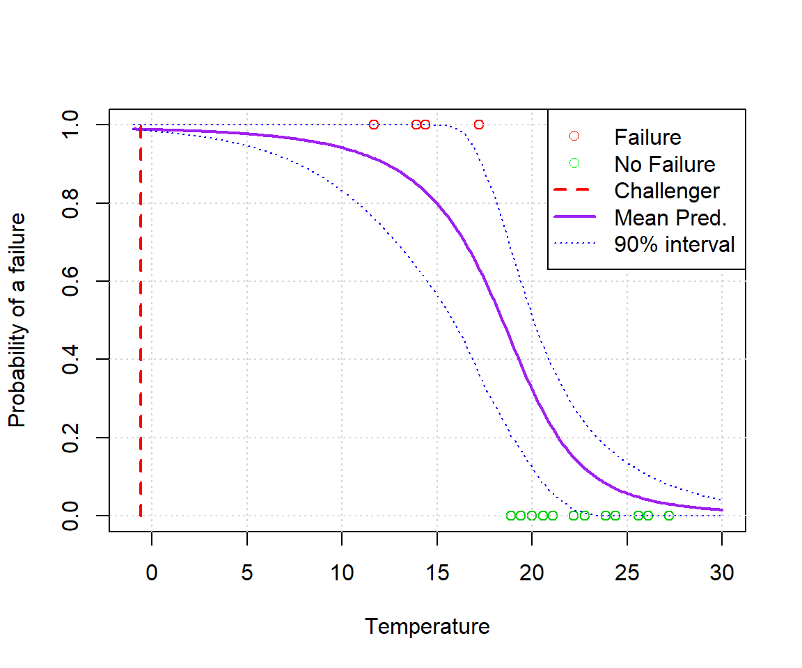

Clearly they should have seen this coming. You don’t need Stan to notice the pattern here.

Tweaking the priors

Suppose we are not happy with the number of green dots outside the prediction interval at the bottom. Let’s try to introduce a prior to adjust it. This is bad statistics in this case, but a fun example nonetheless.

//
// This Stan program defines a basic logistic regression with a single predictor.
// The code below is by Sean van der Merwe, UFS
//
// The input data is a vector 'y', its length 'n', and its explanatory predictor 'x'.
data {
  int<lower=0> n;                   // number of observations
  vector[n] x;                        // explanatory variable
  int<lower=0,upper=1> y[n];  // dependent variable
}
// The parameters accepted by the model.
parameters {
  real beta0;                 // intercept
  real beta1;                 // slope
}
// The model to be estimated.
model {
  y ~ bernoulli_logit(beta0 + beta1 * x);
  beta0 ~ normal(20,5);
  beta1 ~ normal(-3,1);
}

stan_data2 <- list(y=alldata$fail.field, n=n, x=alldata$temp)
fit2 <- sampling(logistic2, stan_data2, pars=c('beta0','beta1'), iter = 32000, chains = 3)
list_of_draws2 <- extract(fit2)

xvals <- seq(-1, 30, l=200)
linpred2 <- c(list_of_draws2$beta1)%*%t(xvals) + c(list_of_draws2$beta0)
ppred2 <- plogis(linpred2)
ppredsummary2 <- apply(ppred2,2,function(x){ c(mean(x),hpd.interval(x,alpha)) })

plot(alldata$temp,alldata$fail.field, xlab='Temperature', ylab='Probability of a failure', xlim=c(min(xvals),max(xvals)), col=(3-alldata$fail.field))
grid()
lines(xvals, ppredsummary2[1,], lwd=2, lty=1, col='purple')
lines(xvals, ppredsummary2[2,], lwd=1, lty=3, col='blue')
lines(xvals, ppredsummary2[3,], lwd=1, lty=3, col='blue')
lines(c(-0.6,-0.6),c(0,1),lwd=2,lty=2,col='red')
legend('topright', c('Failure','No Failure','Challenger','Mean Pred.','90% interval'), lwd=c(0,0,2,2,1), lty=c(0,0,2,1,3), col=c('red','green','red','purple','blue'), pch=c(1,1,NA,NA,NA))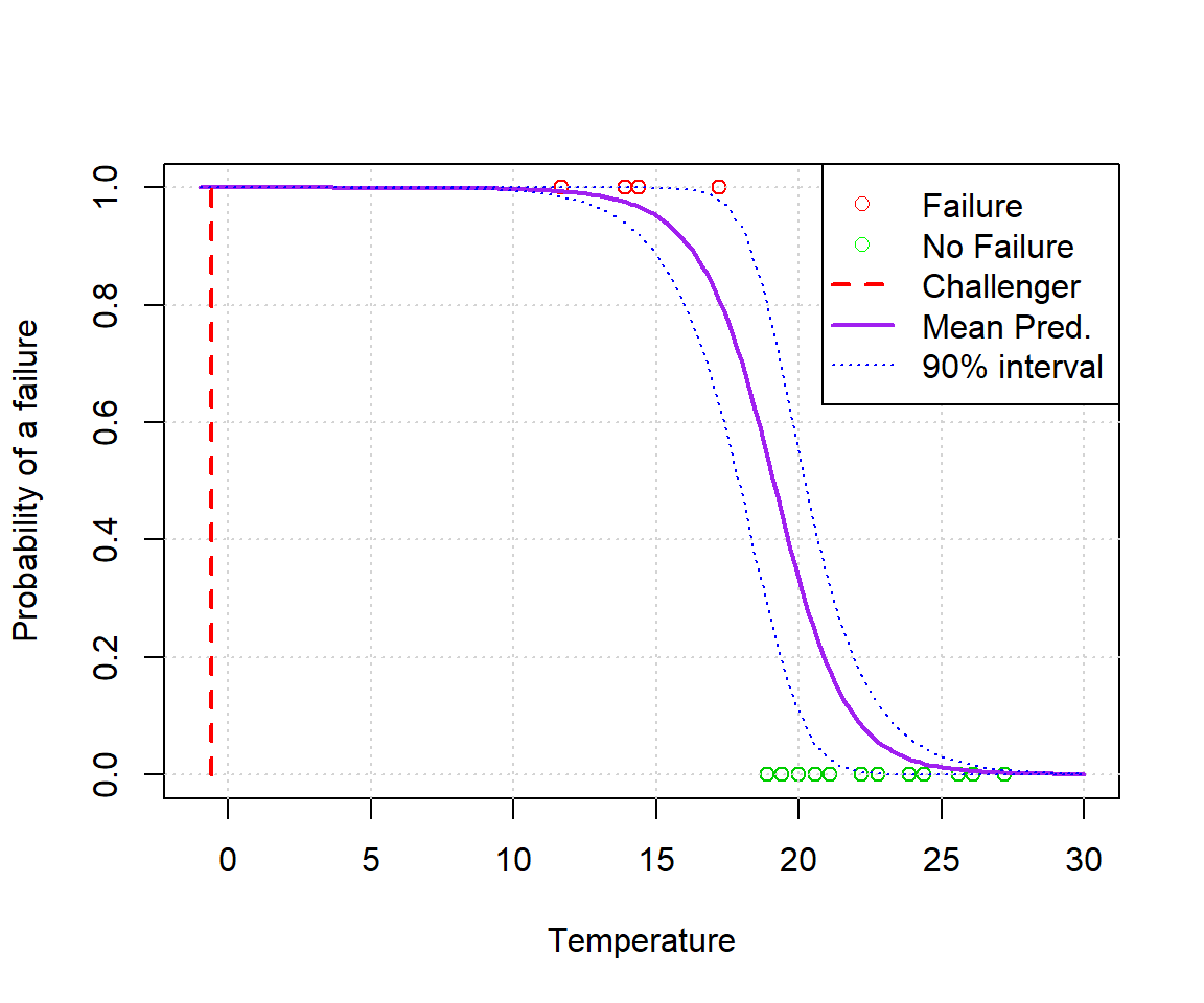

What we see is that even though we tried hard to mess with the model, we’ve only really succeeded in making the bounds smaller (because we introduced additional information).