Introduction
First we read in the data
library(openxlsx)
sourcedata <- read.xlsx('IBM19891998.xlsx')
lret <- sourcedata$LogReturns
dates <- sourcedata$year + sourcedata$month/12 + sourcedata$day/365
Then we plot the data
library(viridisLite)
cols <- viridis(3)
par(mfrow=c(2,1), mar=c(4,4,2,0.2))
plot(dates, lret, type='l', col=cols[1], lwd=1, xlab='Date', ylab='Log return', main='IBM')
hist(lret, 50, col=cols[2], density = 20, ylab='Frequency', xlab='Log return', main='IBM')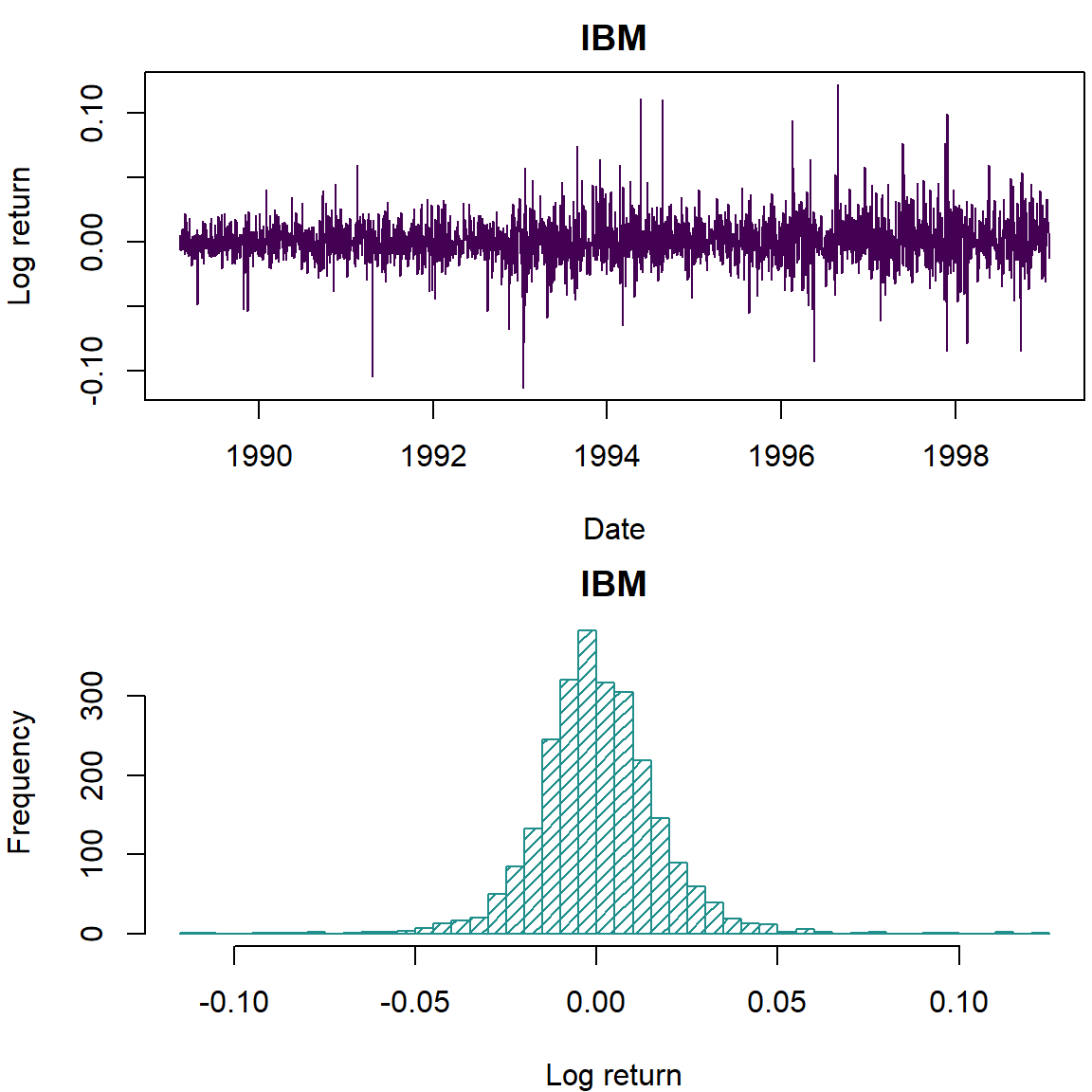
Stan
The new way to fit statistical models is the STAN interface. We will attempt to use this interface via RSTAN to implement our models.
# library(rstan)
# options(mc.cores = 3)
# rstan_options(auto_write = TRUE)

library(parallel); mycores <- max(1,floor(0.75*detectCores(logical = FALSE))) # Choose the number of computer cores to use, 75% of capacity is a good rule of thumb
suppressPackageStartupMessages(library(rstan,warn.conflicts=FALSE,quietly=TRUE))
options(mc.cores = mycores)
rstan_options(auto_write = TRUE)
The basic t model
We define the model in its own block and give it a name
The notation for this is to put {stan, output.var=‘studentt’} as the block header instead of the usual {r studentt}.
//
// This Stan program defines a t fit to a vector of observations.
// The code below is by Sean van der Merwe, UFS
//
// The input data is a vector 'x' and its length 'n'.
data {
  int<lower=0> n;                   // number of observations
  vector[n] x;                        // log of observations
}
// The parameters accepted by the model.
parameters {
  real<lower=0> v;            // degrees of freedom
  real<lower=0> s;            // scale parameter
  real mu;                    // location parameter
}
// The model to be estimated.
model {
  x ~ student_t(v,mu,s);
  v ~ exponential(0.01);
}
Then we run the model
stan_data <- list(x=lret, n=length(lret)) # Create the data list

fitML1 <- optimizing(studentt, stan_data)  # ML estimation

fitBayes1 <- sampling(studentt, stan_data, pars=c('mu','s','v'), iter = 18000, chains = mycores) # Simulation

list_of_draws1 <- extract(fitBayes1) # Extract simulations
saveRDS(list_of_draws1,'studenttIBM1.Rds') # Save simulations
Lastly we plot the results
cols=viridis(6)
par(mfrow=c(2,2), mar=c(4,4,2,0.2))
plot(density(list_of_draws1$v),xlab='v',ylab='Posterior density',main='',col=cols[1],lwd=2)
plot(density(list_of_draws1$s),xlab='s',ylab='Posterior density',main='',col=cols[2],lwd=2)
plot(density(list_of_draws1$mu),xlab='mu',ylab='Posterior density',main='',col=cols[3],lwd=2)

# Posterior Predictive Distribution
postpred1 <- rt(length(list_of_draws1$mu),list_of_draws1$v)*list_of_draws1$s + list_of_draws1$mu
plot(density(postpred1),xlab='Future values',ylab='Posterior density',main='',col=cols[4],lwd=2)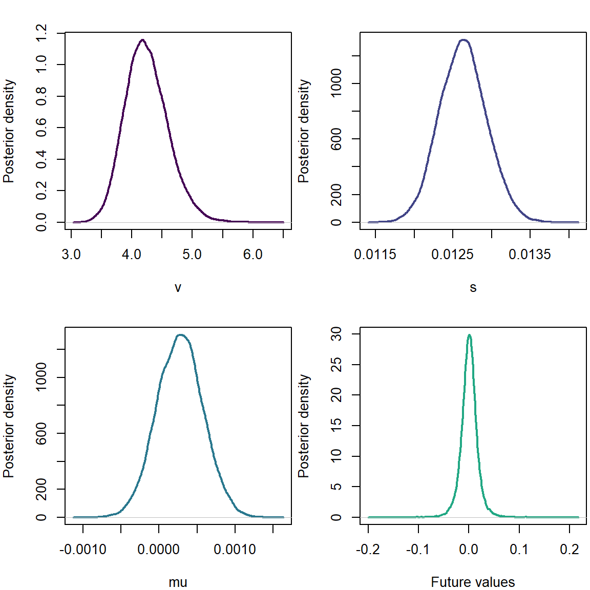
We note a positive mean parameter.
The more advanced skew t model
//
// This Stan program defines a skew t fit to a vector of observations.
// The code below is by Sean van der Merwe, UFS
//
// The input data is a vector 'x' and its length 'n'.
data {
  int<lower=0> n;                   // number of observations
  vector[n] x;                        // log of observations
}
// The parameters accepted by the model.
parameters {
  real<lower=0> v;            // degrees of freedom
  real<lower=0> s;            // scale parameter
  real d;                     // skewness parameter
  real mu;                    // location parameter
  vector<lower=0>[n] z;         // weights of skewness
}
transformed parameters {
  vector[n] mushift;
  mushift = mu + d * z;
}
// The model to be estimated.
model {
  for (i in 1:n)
    z[i] ~ normal(0,1) T[0,];
  x ~ student_t(v,mushift,s);
  v ~ exponential(0.1);
}
stan_data <- list(x=lret, n=length(lret))
# fit <- optimizing(skewt, stan_data)
# print(fit$par[1:4])
fit <- sampling(skewt, stan_data, pars=c('mu','s','v','d'), iter = 8000, chains = mycores)
list_of_draws <- extract(fit)
saveRDS(list_of_draws,'skewtIBM1.Rds')cols=viridis(6)
par(mfrow=c(2,2), mar=c(4,4,2,0.2))
plot(density(list_of_draws$v),xlab='v',ylab='Posterior density',main='',col=cols[1],lwd=2)
plot(density(list_of_draws$d),xlab='d',ylab='Posterior density',main='',col=cols[2],lwd=2)
plot(density(list_of_draws$s),xlab='s',ylab='Posterior density',main='',col=cols[3],lwd=2)
plot(density(list_of_draws$mu),xlab='mu',ylab='Posterior density',main='',col=cols[4],lwd=2)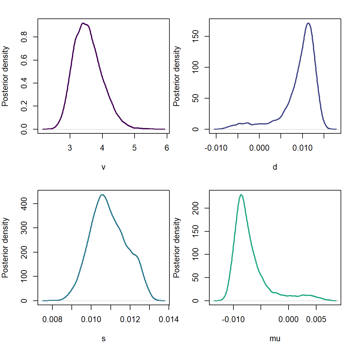
Here we note a positive skewness and a negative mean parameter.
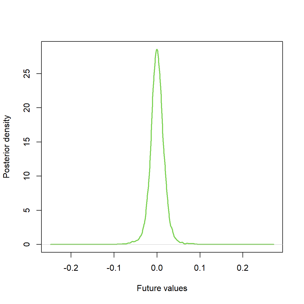
# Posterior Predictive Distribution
postpred <- rt(length(list_of_draws$mu),list_of_draws$v)*list_of_draws$s + list_of_draws$mu + list_of_draws$d*abs(rnorm(length(list_of_draws$mu)))
plot(density(postpred),xlab='Future values',ylab='Posterior density',main='',col=cols[5],lwd=2)