Currently marking student 2001234567
# This code block (if run manually) generates an Excel file with different data for each student according to the list of student numbers

# In this case the data is for a regression with one significant explanatory variable and one irrelevant variable

library(openxlsx)
students <- c(2001234567,2012345678,2000000123)
nStudents <- length(students)
n <- 100
datasets <- vector('list',nStudents)
for (i in 1:nStudents) {
  x1 <- rnorm(n,4,1)
  x2 <- rgamma(n,4,2)
  y <- 20 + 2*x1 + rnorm(n)
  datasets[[i]] <- data.frame(y,x1,x2)
}
names(datasets) <- paste0('St',students)
write.xlsx(datasets, file = "Practical1data.xlsx")
Instructions
Your individual task with this assignment is to build a linear model and discuss it.
- Read in the data from the sheet with your student number and verify that it was read in correctly.
- Fit the standard linear regression model using main effects only, and give the summary.
- Test the individual coefficients for significance if appropriate after testing the global hypothesis.
- Add a scatterplot of \(y\) versus \(x_1\) with the regression line added.
The model is:
\[y_i\sim N(\beta_0+\beta_1x_i,\ \sigma^2)\] ## Memorandum
Q1: Read data
library(openxlsx)
mydata <- read.xlsx('Practical1data.xlsx',paste0('St',params$st))
head(mydata)
## y x1 x2
## 1 29.19206 3.378293 1.7129169
## 2 28.64691 3.651103 1.4887481
## 3 23.59713 2.398480 0.4670791
## 4 29.88086 5.019538 3.5013878
## 5 28.85903 3.502479 1.8389115
## 6 26.96845 4.123522 2.5438280|| 1 mark for reading in their own data. 1 mark for checking it. ||
Q2: Linear model
(s1 <- summary(model1 <- lm(y~x1+x2, data=mydata)))##
## Call:
## lm(formula = y ~ x1 + x2, data = mydata)
##
## Residuals:
## Min 1Q Median 3Q Max
## -3.00376 -0.64894 -0.05359 0.80885 2.27539
##
## Coefficients:
## Estimate Std. Error t value Pr(>|t|)
## (Intercept) 20.1353 0.4720 42.661 <2e-16 ***
## x1 1.9209 0.1077 17.844 <2e-16 ***
## x2 0.1705 0.1215 1.404 0.164
## ---
## Signif. codes: 0 '***' 0.001 '**' 0.01 '*' 0.05 '.' 0.1 ' ' 1
##
## Residual standard error: 1.07 on 97 degrees of freedom
## Multiple R-squared: 0.7689, Adjusted R-squared: 0.7641
## F-statistic: 161.4 on 2 and 97 DF, p-value: < 2.2e-16Q3: Model discussion
In order to test the global hypothesis that no coefficients are significant we look at the F test p-value. If it is more than \(\alpha\) we fail to reject the global null hypothesis and stop there. If the p-value is significant (\(<\alpha\)) then we test the individual hypotheses.
|| 2 marks for having a global conclusion, and discussing it. ||
The individual hypothesis is simply \(H_0:\beta_i=0\ vs\ H_1:\beta_i\ne 0\). We reject the individual hypothesis for the significant terms based on the original p-values being less than \(\alpha\) and conclude that these terms are useful and significant in predicting \(y\).
|| 4 marks for discussing individual terms if appropriate. ||
Q4: Plot
plot(mydata$x1, mydata$y, pch=4, col='purple', main = '', xlab = expression(x[1]), ylab = expression(y))
abline(coef(model1)[1:2], col='blue', lwd=2, lty=4)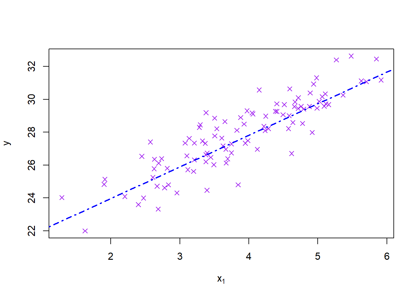
|| 2 marks for neat plot with line. ||
|| Total: 10 marks ||