Observed data
We begin by reading in data. We will use the old FTSE stock exchange index for this example. We will try to reach stationarity via calculating log returns.
data(EuStockMarkets)
Index <- EuStockMarkets[,'FTSE']
n <- length(Index)
LogReturns <- diff(log(Index))
n1 <- length(LogReturns)
par(mfrow=c(1,2),bg=rgb(0,0,0),fg=rgb(1,1,1),col.axis='white',col.main='white',col.lab='white',mar=c(4,4,0.6,0.2))
plot(Index,col='#2A9FD6',lwd=2)
plot(LogReturns,col='#2A9FD6')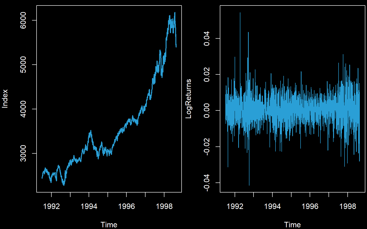
Next we consider any residual correlation.
source('autocor.r')
par(mfrow=c(1,2),bg=rgb(0,0,0),fg=rgb(1,1,1),col.axis='white',col.main='white',col.lab='white',mar=c(4,4,0.6,0.2))
autocor(LogReturns)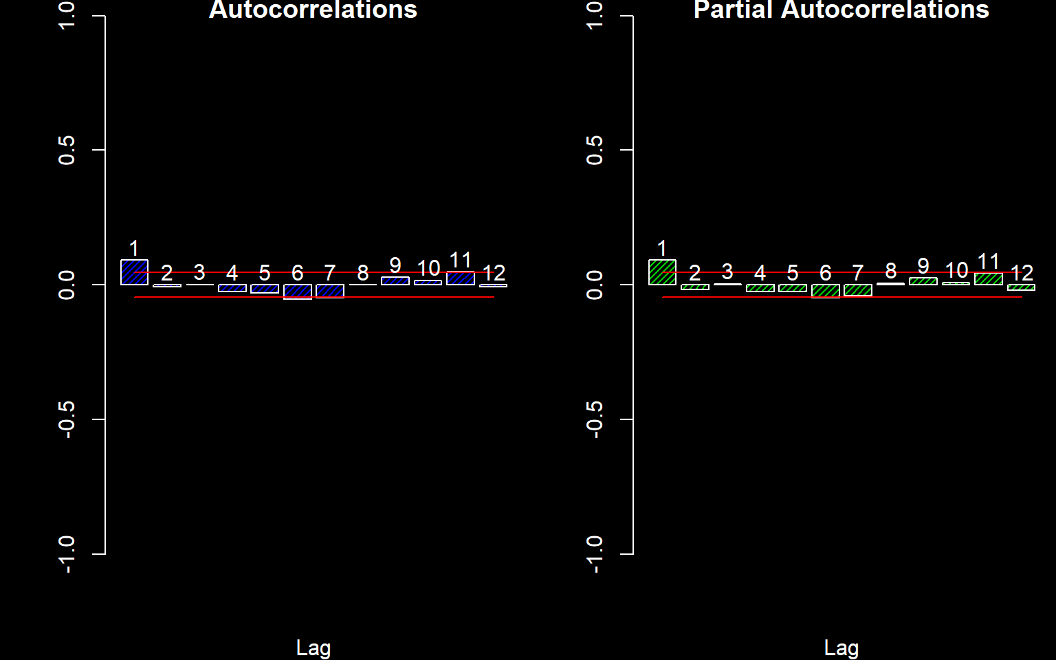
##             Autocor Partial Autocor
##  [1,]  0.0920293254     0.092029325
##  [2,] -0.0080311473    -0.016641487
##  [3,]  0.0010092917     0.003321238
##  [4,] -0.0243573941    -0.025113544
##  [5,] -0.0299437221    -0.025526611
##  [6,] -0.0520103747    -0.047963033
##  [7,] -0.0472235819    -0.039074571
##  [8,] -0.0003064717     0.005856628
##  [9,]  0.0279680560     0.025664810
## [10,]  0.0157556291     0.008441719
## [11,]  0.0486153284     0.043330682
## [12,] -0.0066226871    -0.019355528
There appears to be some correlation at Lag 1. We will fit an AR(1) model assuming normal residuals. This is not the optimal model but will do for now.
(model <- arima(LogReturns,c(1,0,0)))##
## Call:
## arima(x = LogReturns, order = c(1, 0, 0))
##
## Coefficients:
## ar1 intercept
## 0.0921 4e-04
## s.e. 0.0231 2e-04
##
## sigma^2 estimated as 6.275e-05: log likelihood = 6356.29, aic = -12706.58r <- resid(model)
Box.test(r,12,'Ljung-Box')##
## Box-Ljung test
##
## data: r
## X-squared = 16.324, df = 12, p-value = 0.1768As the coefficient appear significant and the Box test fails to reject white noise, we will use this model for now (even though the residuals are not actually white noise).
We must fit a distribution to the residuals. We draw a histogram and decide on a valid model.
par(bg=rgb(0,0,0),fg=rgb(1,1,1),col.axis='white',col.main='white',col.lab='white',mar=c(4,4,0.6,0.2))
hist(r,20,col='#2A9FD6',density = 20)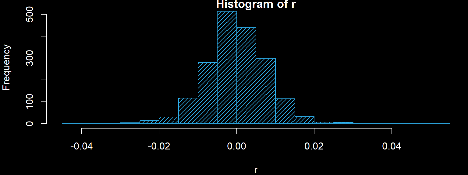
shapiro.test(r)##
## Shapiro-Wilk normality test
##
## data: r
## W = 0.98186, p-value = 1.308e-14The Shapiro-Wilk test rejects normality, so we try a t-distribution.
library(MASS)
f <- fitdistr(r,'t')
(Parests.t <- coef(f))
## m s df
## -0.0000028712 0.0067170394 7.1867819910(Sigma.t <- vcov(f))## m s df
## m 3.024467e-08 -1.327690e-10 -9.072518e-07
## s -1.327690e-10 2.800347e-08 1.212649e-04
## df -9.072518e-07 1.212649e-04 1.148705e+00Prediction
In order to predict the next \(m\) time periods, we proceed as follows:
- Pick the number of paths to simulate, call it \(K\).
- Simulate \(K\) sets of model parameters taking into account the uncertainty in the parameter estimation. Do this for both the residual model and the stationary model.
- For each set of model parameters predict the next \(m\) residual values.
- Iteratively plug then into the stationary model using the corresponding coefficients to get predictions for the log returns.
m <- 24
K <- 10000
Pars.t <- mvrnorm(K,Parests.t,Sigma.t)
Pars.model <- mvrnorm(K,coef(model),vcov(model))
PredMat <- matrix(0,K,m)
for (j in 1:K) {
  PredMat[j,1] <- Pars.model[j,] %*% c(LogReturns[n1],1) + rt(1,Pars.t[j,3])*Pars.t[j,2]+Pars.t[j,1]
  for (i in 2:m) {
    PredMat[j,i] <- Pars.model[j,] %*% c(PredMat[j,(i-1)],1) + rt(1,Pars.t[j,3])*Pars.t[j,2]+Pars.t[j,1]
  }
}
We can then reverse the transformations in order to predict the Index values.
FinalLogObs <- log(Index[n])
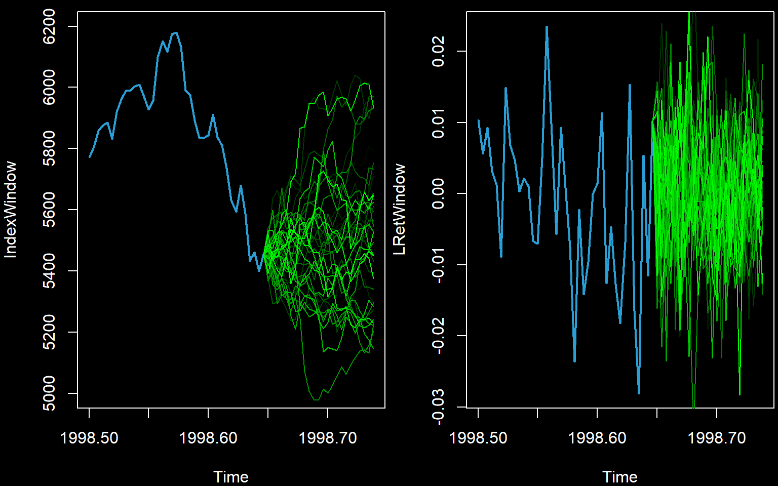
IndexPred <- t(apply(PredMat,1,function(x){ exp(cumsum(x)+FinalLogObs) }))Now we must illustrate the predictions. We will first illustrate the simulated paths. This is not the standard way to illustrate predictions but aids understanding.
We zoom in to show the last part of the series only. We show only the first few paths.
numpathstoshow <- 40
startingpoint <- round(n*0.8)
newtimes <- (0:m)/frequency(Index) + time(Index)[n]
par(mfrow=c(1,2),bg=rgb(0,0,0),fg=rgb(1,1,1),col.axis='white',col.main='white',col.lab='white',mar=c(4,4,0.6,0.2))
IndexWindow <- window(Index,start=1998.5)
plot(IndexWindow,col='#2A9FD6',lwd=2,xlim=c(min(time(IndexWindow)),max(newtimes)),ylim=c(5000,6200))
for (j in 1:numpathstoshow) {
  lines(newtimes,c(Index[n],IndexPred[j,]),lwd=1,col=rgb(0,j/numpathstoshow,0))
}
LRetWindow <- window(LogReturns,start=1998.5)
plot(LRetWindow,col='#2A9FD6',lwd=2,xlim=c(min(time(LRetWindow)),max(newtimes)))
for (j in 1:numpathstoshow) {
  lines(newtimes,c(LogReturns[n1],PredMat[j,]),lwd=1,col=rgb(0,j/numpathstoshow,0))
}
The standard way is via means and prediction intervals (which must first be calculated from the predicted paths).
Index.Int <- apply(IndexPred,2,quantile,c(0.025,0.975))
Index.Pred <- colMeans(IndexPred)
LRet.Int <- apply(PredMat,2,quantile,c(0.025,0.975))
LRet.Pred <- colMeans(PredMat)
par(mfrow=c(1,2),bg=rgb(0,0,0),fg=rgb(1,1,1),col.axis='white',col.main='white',col.lab='white',mar=c(4,4,0.6,0.2))
plot(IndexWindow,col='#2A9FD6',lwd=2,xlim=c(min(time(IndexWindow)),max(newtimes)),ylim=c(5000,6200))
lines(newtimes,c(Index[n],Index.Pred),lwd=2,col=rgb(1,1,0))
lines(newtimes,c(Index[n],Index.Int[1,]),lwd=2,col=rgb(0,1,0))
lines(newtimes,c(Index[n],Index.Int[2,]),lwd=2,col=rgb(0,1,0))

plot(LRetWindow,col='#2A9FD6',lwd=2,xlim=c(min(time(LRetWindow)),max(newtimes)))
lines(newtimes,c(LogReturns[n1],LRet.Pred),lwd=2,col=rgb(1,1,0))
lines(newtimes,c(LogReturns[n1],LRet.Int[1,]),lwd=2,col=rgb(0,1,0))
lines(newtimes,c(LogReturns[n1],LRet.Int[2,]),lwd=2,col=rgb(0,1,0))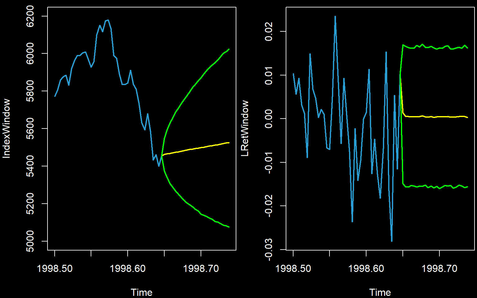
Theoretical approach
It is worth noting that these lines and intervals are not as accurate nor as smooth as those calculated using theory.
The basic principle behind the theoretical approach for an AR(1) model is as follows:
- Assume independent residuals with mean zero and constant variance \(\sigma^2_e\). Remember that everything up to time \(n\) is given.
- \(X_{n+1}=\mu+\phi X_{n}+\varepsilon_{n+1}\)
- \(E[X_{n+1}]=\mu+\phi X_{n}+E[\varepsilon_{n+1}]=\mu+\phi X_{n}+0=\mu+\phi X_{n}\)
- \(X_{n+1}-E[X_{n+1}]=\mu+\phi X_{n}+\varepsilon_{n+1}-(\mu+\phi X_{n})=\varepsilon_{n+1}\)
- \(Var(X_{n+1}-E[X_{n+1}])=Var(\varepsilon_{n+1})=\sigma^2_e\)
- \(E[X_{n+2}]=\mu+\phi E[X_{n+1}]\)
- \(X_{n+2}-E[X_{n+2}]=\mu+\phi X_{n+1}+\varepsilon_{n+2}-(\mu+\phi E[X_{n+1}])=\phi(X_{n+1}-E[X_{n+1}])+\varepsilon_{n+2}=\phi\varepsilon_{n+1}+\varepsilon_{n+2}\)
- \(Var(X_{n+2}-E[X_{n+2}])=Var(\phi\varepsilon_{n+1}+\varepsilon_{n+2})=\phi^2\sigma^2_e +\sigma^2_e=(\phi^2+1)\sigma^2_e\)
- \(E[X_{n+3}]=\mu+\phi E[X_{n+2}]\)
- \(X_{n+3}-E[X_{n+3}]=\mu+\phi X_{n+2}+\varepsilon_{n+3}-(\mu+\phi E[X_{n+2}])=\phi(\phi\varepsilon_{n+1}+\varepsilon_{n+2})+\varepsilon_{n+3}=\phi^2\varepsilon_{n+1}+\phi\varepsilon_{n+2}+\varepsilon_{n+3}\)
- \(Var(X_{n+3}-E[X_{n+3}])=Var(\phi^2\varepsilon_{n+1}+\phi\varepsilon_{n+2}+\varepsilon_{n+3})=(\phi^4+\phi^2+1)\sigma^2_e\)
- etc.
The above derivations differ for every type of model.