What are we doing and why?
We are just going to draw a graph in R with multiple lines on one graph. This is interesting because the way base R draws graphs is a bit strange to people who are used to other packages. Some explanation is useful.
Specific example
In this example we are going to use the lengths of the 25 most popular movies of each year from 1931 to 2013, as explained here bu Randy Olson.
The raw data is available on his site. The transformed data is here.
Read data
First we read in the data and create named variables to work with.
mydata <- read.csv('filmlengthsratings.csv')
names(mydata)
## [1] "Film" "Year" "Rating" "Number_Ratings"
## [5] "Length_Minutes"attach(mydata)Calculation of intervals
We are just going to make standard 95% t intervals, based on the assumption of Normality.
L <- Length_Minutes
means <- tapply(L,Year,mean)
sds <- tapply(L,Year,sd)
ns <- tapply(L,Year,length)
Lower <- means - qt(0.975,ns-1)*sds/sqrt(ns)
Upper <- means + qt(0.975,ns-1)*sds/sqrt(ns)
Drawing the graph
We can start with a windows command to make an empty window of the correct size, e.g. windows(8,5).
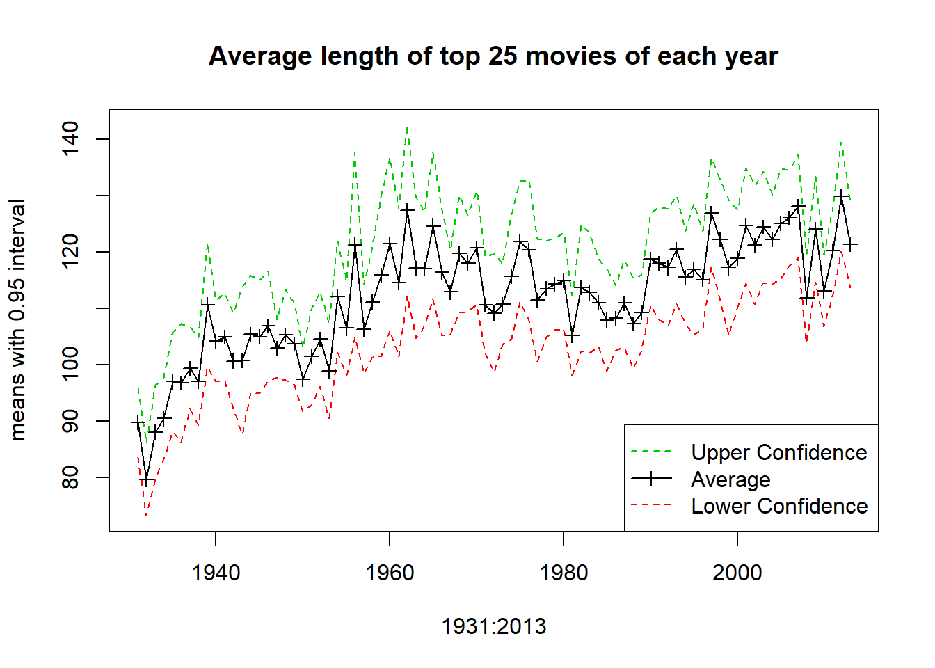
Then we plot the basic graph, and use lines to add lines, or points to add points. Note the use of ylim to ensure there is enough space on the graph for all the lines.
plot(1931:2013,means,type='l', main="Average length of top 25 movies of each year", ylim=c(min(Lower),max(Upper)), ylab='means with 0.95 interval')
lines(1931:2013,Lower,col=2,lty=2)
lines(1931:2013,Upper,col=3,lty=2)
points(1931:2013,means,pch=3)
legend('bottomright',c('Upper Confidence','Average','Lower Confidence'), col=c(3,1,2),lty=c(2,1,2),pch=c(NA,3,NA))