Simulating an ARIMA Time Series

Step 1: How long must the time series be?

Begin by deciding on a reasonable length for your time series, based on the problem at hand.

Then add a burn-in period: that is an extra piece that we add at the start of the time series while simulating but throw away later. When you simulate a time series the first part you simulate will not follow your chosen model and must be discarded.

chosen.length <- 200; burnin <- 100
n <- chosen.length + burnin

Step 2: White Noise

Simulation of an ARIMA series begins with the uncorrelated random errors. These may follow any distribution, but they should be independent and identically distributed.

The simplest option is using a standard Normal distribution (Gaussian white noise), but this can cause problems if you series is restricted.

To simulate from a standard distribution in R the command is the letter r followed by the short name of the distribution that R uses. Then we provide the number of observations to simulate, followed by the parameter values. Remember that R might define the parameters differently to what you are used to! Always check the help.

?rnorm

## starting httpd help server ... done

e <- rnorm(n,0,1)

Step 3: Make room

Next we create space for storing our time series. This ensures smooth execution. We can create an empty vector, or just copy the random errors we generated since they are already the correct length.

x <- e

Step 4: Select parameter values

Assuming we know what model we wish to simulate, we must now select reasonable values for the parameters.

In this example we are going to simulate an ARIMA(2,1,1) model. Adapt the code to suit your model, which will be different.

I am going to select parameters of \(\mu=0.2\), \(\phi_1=0.3\), \(\phi_2=0.4\), \(\theta_1=0.5\), and \(\sigma=1.2\). These parameters result in a stationary model, which is essential.

If you are not sure whether you have chosen valid parameters then set up and solve the auxilliary equation to check.

mu <- 0.2; phi1 <- 0.3; phi2 <- 0.4; theta1 <- 0.5; sigma <- 1.2

Step 5: Generate series

Now we can generate our series. This must be doing in a loop because a time series develops iteratively over time. The inside of the loop contains your chosen model, which must be adapted every time the model changes.

Note that the loop must start at a number higher than the largest lag in the model (so that you don’t go into negative time).

for (i in 3:n) {
  x[i] <- mu + phi1*x[i-1] + phi2*x[i-2] + sigma*e[i] - theta1*e[i-1]
}

Step 6: Order of integration

The order of integration is the number of times a series must be differenced to be stationary. We have generated a stationary series, so it’s the number of times we must reverse-difference our stationary series in order to arrive at the target model. The opposite of difference is sum, specifically the cumulative sum.

In this case we need to sum once because we have \(d=1\) in this example.

Sx <- cumsum(x)

Step 7: Discard burn-in period

The start of the generated time series does not fit our target model and must be discarded. We thus keep the part of the time series after the burn-in period.

y <- Sx[(burnin+1):n]

Step 8: Make it a time series

Right now we just have a vector of numbers. We now turn this into a time series. Optionally: We can specify a start time and frequency to give our time series a nice scale.

In this example we will assume we have a monthly series spanning nearly 17 years.

y <- ts(y, start=2001.5,frequency = 12)

Step 9: Check that the series looks right

We use plots and correlograms to do a basic check that we met our goal of simulating from the target model. The most important is a plot of the final series we produced.

plot(y,main='ARIMA(2,1,1)',xlab = 'Time',ylab='Series values',col='purple',lwd=2)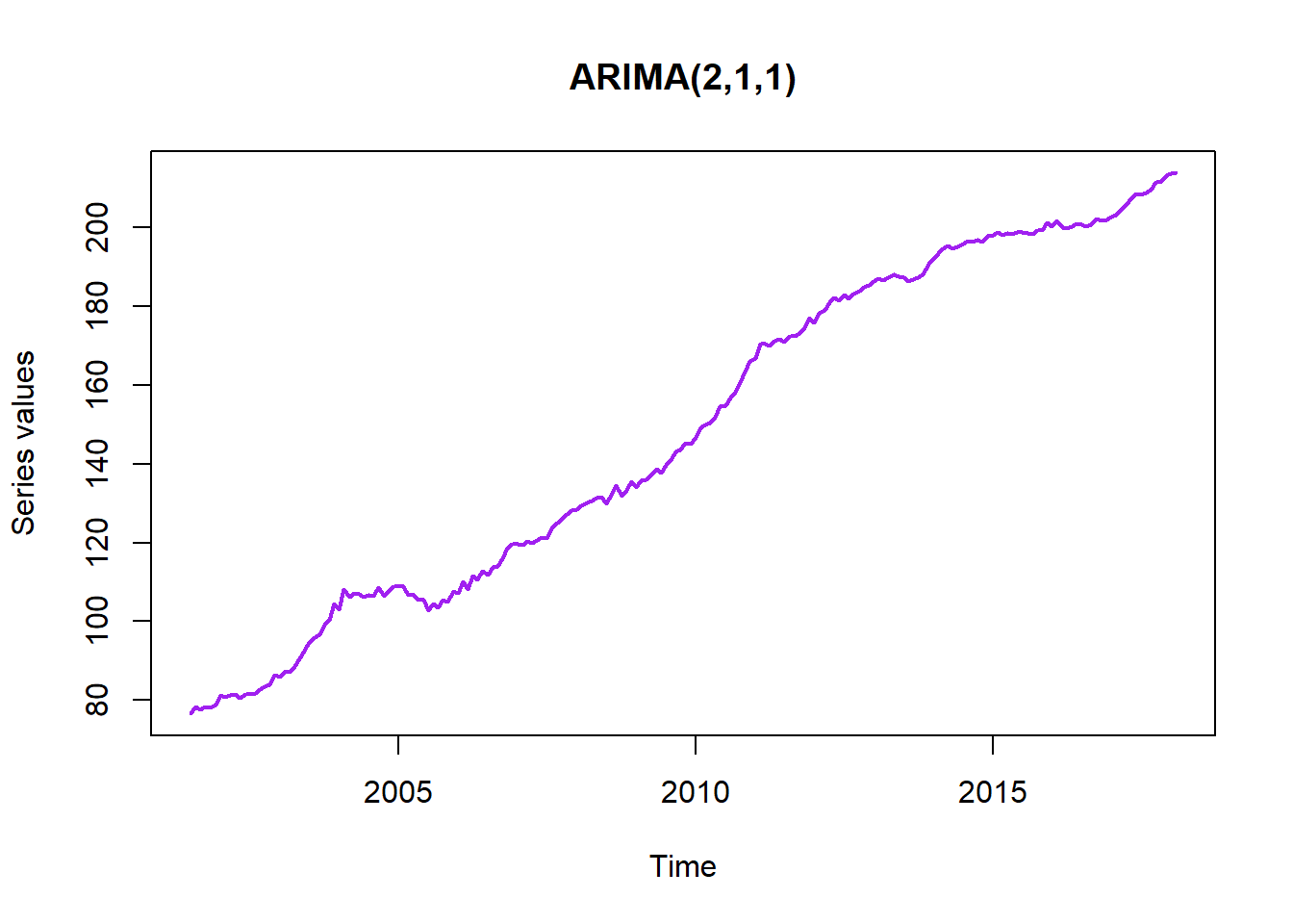

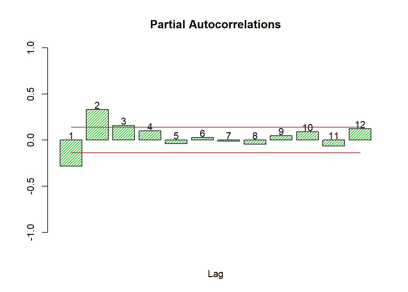
Additionally we can draw correlograms of the stationary series and see if they seem reasonable for our model.

DY <- diff(y)
source('autocor.r')
cors <- autocor(DY)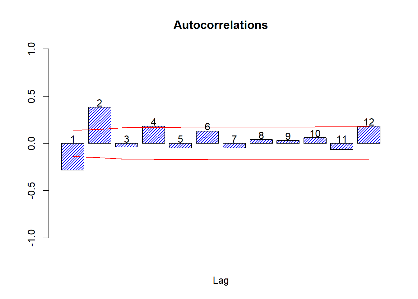

Step 10: Report our generated series

It’s a good idea to save our series in a standard format like a .csv file.

write.csv(y,'GenARIMA.csv')

And that’s how you simulate a time series.