Simulation attempt for Andréhette Verster

Introduction and disclaimer

The data simulated here pertains to a specific set of assumptions, and we should not try to extend the results beyond that without seriously considering and accounting for any systematic differences between that situation and any broader situation.

The data analysed here is inherently random. If the study were to be repeated then the results will differ.

While the computer software used is tried and tested, the analysis involves multiple human elements.

Basic data creation

library(viridisLite) # Nicer colour palettes for graphs (optional)
alpha <- 0.1 # The chosen significance level for intervals

We generate some Frechét samples to analyse.

full_sample_size <- 300
nsamples <- 1000
evi_true <- (1/3)
samples_all <- matrix((-log(runif(full_sample_size*nsamples)))^(-evi_true),full_sample_size,nsamples)

The significance level chosen is 0.1. This means that we only look at results where the p-value is less than 0.1, as other results could easily just be chance variation.

The current gold standard for implementing advanced Bayesian models is the STAN interface. We will attempt to use this interface via RSTAN to implement our models.

suppressPackageStartupMessages(library(rstan,warn.conflicts=FALSE,quietly=TRUE))
options(mc.cores = 1)
rstan_options(auto_write = TRUE)

One sample, one threshold

We first define the model for a single threshold.

//
// This Stan program defines a specific generalisation of the Topp-Leone distribution developed by Dr Verster, UFS.
// The code below is by Sean van der Merwe, UFS
//
// The input data is a vector 'ly', its length 'n', and its sum 'sly'. Providing all three is needed for maximum speed.
data {
  int<lower=0> n;                   // number of observations
  vector[n] ly;                       // log of real valued pre-sorted observations
  real sly;                   // sum of ly
}
// The parameters accepted by the model.
parameters {
  real<lower=0> evi;          // extreme value index
  real<lower=0> a;            // shape parameter
}
// The model to be estimated.
model {
  target += (n-1)*(log(a)+log(evi)) - sly*(2*evi+1) + (a-1)*sum(log(1-exp(-2*evi*ly)));
}

Then we prepare the data appropriately and run the model.

x <- sort(samples_all[,1])
x <- x[201:full_sample_size]/x[200]
stan_data <- list(ly=log(x), n=length(x), sly=sum(log(x)))

fit <- sampling(TPverster, stan_data, pars=c('a','evi'), iter = 2000, chains = 1)

## 
## SAMPLING FOR MODEL '4f714613a97978092028111ff7b212d0' NOW (CHAIN 1).
## Chain 1: 
## Chain 1: Gradient evaluation took 0 seconds
## Chain 1: 1000 transitions using 10 leapfrog steps per transition would take 0 seconds.
## Chain 1: Adjust your expectations accordingly!
## Chain 1: 
## Chain 1: 
## Chain 1: Iteration:    1 / 2000 [  0%]  (Warmup)
## Chain 1: Iteration:  200 / 2000 [ 10%]  (Warmup)
## Chain 1: Iteration:  400 / 2000 [ 20%]  (Warmup)
## Chain 1: Iteration:  600 / 2000 [ 30%]  (Warmup)
## Chain 1: Iteration:  800 / 2000 [ 40%]  (Warmup)
## Chain 1: Iteration: 1000 / 2000 [ 50%]  (Warmup)
## Chain 1: Iteration: 1001 / 2000 [ 50%]  (Sampling)
## Chain 1: Iteration: 1200 / 2000 [ 60%]  (Sampling)
## Chain 1: Iteration: 1400 / 2000 [ 70%]  (Sampling)
## Chain 1: Iteration: 1600 / 2000 [ 80%]  (Sampling)
## Chain 1: Iteration: 1800 / 2000 [ 90%]  (Sampling)
## Chain 1: Iteration: 2000 / 2000 [100%]  (Sampling)
## Chain 1: 
## Chain 1:  Elapsed Time: 0.073 seconds (Warm-up)
## Chain 1:                0.071 seconds (Sampling)
## Chain 1:                0.144 seconds (Total)
## Chain 1:

list_of_draws <- extract(fit)
plot(list_of_draws$evi, list_of_draws$a, xlab = 'EVI', ylab = 'a', main = 'Joint Posterior Distribution', pch='.', col='purple')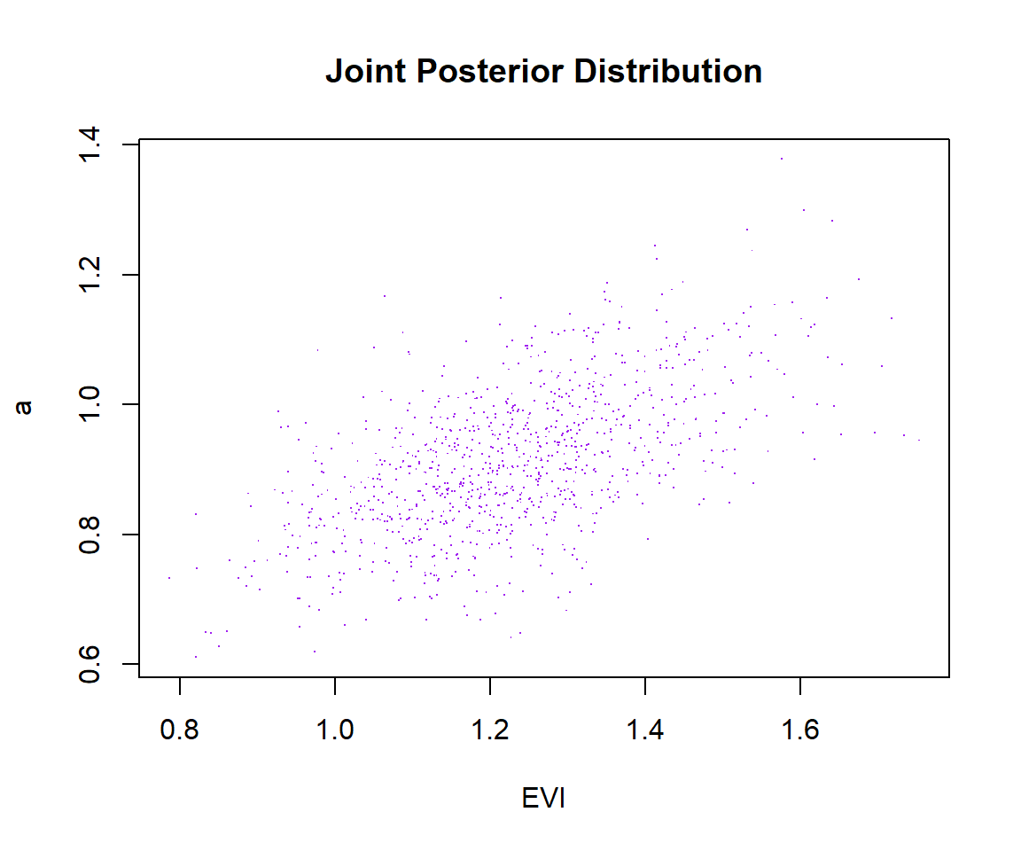

One sample, many thresholds

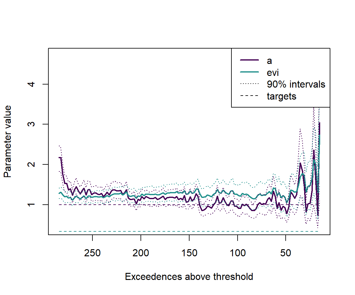
Here we consider thresholds from 5% to 95% of the data, in steps of 2 observations. For each threshold we take the exceedences and divide them by the threshold, fit the model, and return the expected values and intervals of the parameters.

threshold_low <- max(floor(full_sample_size*0.05),10)
threshold_high <- max(floor(full_sample_size*0.95),20)

current_sample <- sort(samples_all[,1])
samplelist <- sapply(seq(threshold_low,threshold_high,2), function(threshold) {
  current_sample[(threshold+1):full_sample_size]/current_sample[threshold]
})

library(parallel)

hpd.interval <- function(postsims,alpha=0.05) { # Coded by Sean van der Merwe, UFS
sorted.postsims <- sort(postsims)
nsims <- length(postsims)
numints <- floor(nsims*alpha)
gap <- round(nsims*(1-alpha))
widths <- sorted.postsims[(1+gap):(numints+gap)] - sorted.postsims[1:numints]
HPD <- sorted.postsims[c(which.min(widths),(which.min(widths) + gap))]
return(HPD) }

runstan1 <- function(x) {
  stan_data <- list(ly=log(x), n=length(x), sly=sum(log(x)))
  fit <- sampling(TPverster, stan_data, pars=c('a','evi'), iter = 2000, chains = 1)
  list_of_draws <- extract(fit)
  results <- c(mean(list_of_draws$a), mean(list_of_draws$evi), hpd.interval(list_of_draws$a,alpha), hpd.interval(list_of_draws$evi,alpha))
  names(results) <- c('a_mean','evi_mean','a_lower','a_upper','evi_lower','evi_upper')
  return(results)
}

Model fitting is done in parallel for faster execution.

cl <- makeCluster(max(floor(0.75*detectCores(logical = FALSE)),1))
nul <- clusterExport(cl,c('alpha','hpd.interval','runstan1','TPverster'))
nul <- clusterEvalQ(cl,{
  suppressPackageStartupMessages(library(rstan,warn.conflicts=FALSE,quietly=TRUE))
  options(mc.cores = 1)
  rstan_options(auto_write = TRUE)
})
outputs <- parLapply(cl,samplelist,runstan1)
stopCluster(cl)

Then we visualise the results:

numexceedences <- unlist(lapply(samplelist,length))
outputs_neat <- t(as.data.frame(outputs,col.names = paste0('ex',numexceedences)))
plot(c(min(numexceedences),max(numexceedences)),c(min(outputs_neat),max(outputs_neat)), type='n', xlab='Exceedences above threshold', ylab='Parameter value', xlim=c(max(numexceedences),min(numexceedences)))
cols <- viridis(3)
lines(numexceedences, outputs_neat[,1], lwd=2, lty=1, col=cols[1])
lines(numexceedences, outputs_neat[,2], lwd=2, lty=1, col=cols[2])
lines(numexceedences, outputs_neat[,3], lwd=1, lty=3, col=cols[1])
lines(numexceedences, outputs_neat[,4], lwd=1, lty=3, col=cols[1])
lines(numexceedences, outputs_neat[,5], lwd=1, lty=3, col=cols[2])
lines(numexceedences, outputs_neat[,6], lwd=1, lty=3, col=cols[2])
lines(numexceedences, rep(1,length(numexceedences)), lwd=1, lty=2, col=cols[1])
lines(numexceedences, rep(evi_true,length(numexceedences)), lwd=1, lty=2, col=cols[2])
legend('topright',c('a','evi','90% intervals','targets'),lwd=c(2,2,1,1),lty=c(1,1,3,2),col=c(cols[c(1,2)],rgb(0,0,0),rgb(0,0,0)))