2021
Introduction
What are Old Wives’ Tales?
Rules or sayings passed down through generations that, to quote Wikipedia, contain “unverified claims with exaggerated and/or inaccurate details.”
Example from my mother: “Don’t pull faces, if the wind changes then your face will stay that way.”
Recently debunked example: “Don’t swim after eating - you can get stomach cramps.”
Often they are created with good reasons, like parents wanting to rest after eating and not watch their kids in the pool.
And often those reasons are lost over time, leaving only a rule without context. Then when the context changes the rule stops being valid without people realising it.
What about statistics?
In statistics we also have many rules that are sometimes taught as hard rules, but were actually never meant to be more than temporary rules of thumb.
Or rules that were actually twisted over time from good intentions, through misunderstandings, to end up being quite wrong or bad practice.
And of course rules that were created in times before computing power and Big Data where the authors never conceived of the idea that I’d have a personal computer at home that can perform 100,000 t-tests per second.
Outline for this talk
- Sample size greater than 30 matters
- Variance test before t-test
- The data should be normal
- A p-value tells you about the alternative
- The number of tests you did isn’t relevant, and neither are the insignificant ones you didn’t show
- R-square is a good measure of model fit and is very useful for exploratory modelling
- The drive for reproducible and open research is a nuisance
- Use the same data to test a model you built for it
Hypothesis testing
General idea
- Assume the world is boring
- See something possibly interesting
- Work out how likely it is to see something at least that interesting under the assumption that the world is boring
- This is called a p-value
- If the p-value is large (say more than 0.05) then we keep assuming the world is boring
- If the p-value is small (say less than 0.05) then we reject our assumption that the world is boring and conclude there’s at least one interesting thing going on
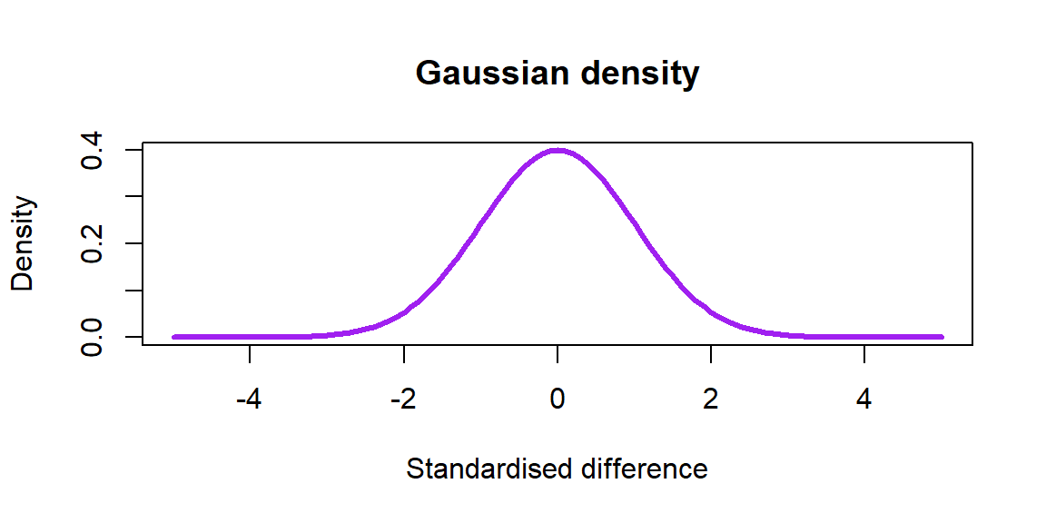
Distributions
- The Central Limit Theorem says that averages follow a Gaussian (Normal) distribution
- IF your sample size is large enough
- So if we care about the average then we can make judgements using this theorem
t-test
- The t-test seems to be the most popular tool in statistics after summary statistics and graphs
- Assuming you are interested in testing some hypothesized average \((\mu)\)
- Usually “No difference”, implying an average difference of zero \((\mu=0)\)
- IF your sample size is large enough then
- \(t=\)(The average minus \(\mu\))*\(\sqrt{n}\)/standard deviation
- Follows a \(t_{n-1}\) distribution in a boring world, where \(n\) is the number of observations
- So if \(|t|\) is large (>2 is a good rule of thumb) then we reject the boring hypothesis
So what’s the problem?
- A long time ago the only practical way to do a t-test was with tables of critical values.
- Normal tables were markedly more accurate than t-tables.
- As the degrees of freedom of the t density increases then it approaches the normal density.
- So people chose a point \((n=30)\) where they would switch from the t-table to the normal table.
- Students were taught this rule of thumb, but instead of understanding it, they just memorised it (as students are prone to do).
- Those students then became professors and taught the next generation.
- And to this day people are taught to use a z-table for \(n>30\).
- This is a needless waste of teaching time and brain power as we can now just teach students to do a t-test in all cases. The sample size stops being an issue, and it takes an equal amount of time on the computer (about 0.0001 seconds).
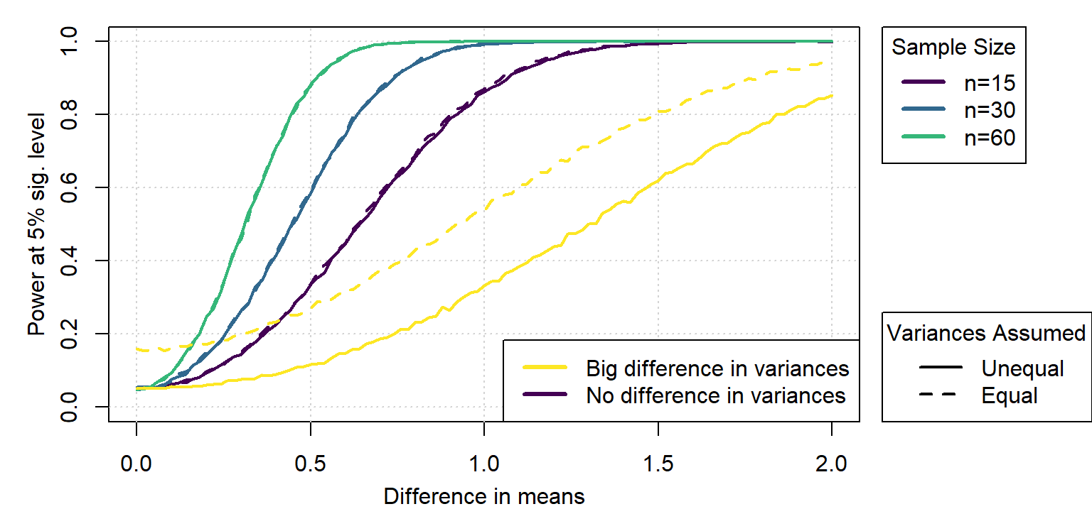
Variance test then t-test
- It is standard practice in many places to do a test for equality of variances before doing a two sample t-test.
- If the variance test fails to reject then people do an equal variance t-test, and if it rejects then people do an unequal variance t-test.
- I also engaged in and taught this practice on occasion in the past.
But I will show you now that it is a waste of time and effort.
Just do the unequal variance test every time.
Simulation study
Let’s look at the power of the t-test in both cases via simulation study. This is not a very good or neat example of a simulation study, but it will do for this presentation.
alpha <- 0.05
pwrequal <- function(mudif, n) {
    mean(replicate(10000, t.test(rnorm(n, mudif, 1), rnorm(n),
        var.equal = TRUE)$p.value) < alpha)
}
pwr <- function(mudif, n) {
    mean(replicate(10000, t.test(rnorm(n, mudif, 1), rnorm(n))$p.value) <
        alpha)
}
mudif <- seq(0, 2, l = 101)
pwrcurve15 <- sapply(mudif, pwr, n = 15)
pwrequalcurve15 <- sapply(mudif, pwrequal, n = 15)
pwrcurve30 <- sapply(mudif, pwr, n = 30)
pwrequalcurve30 <- sapply(mudif, pwrequal, n = 30)
pwrcurve60 <- sapply(mudif, pwr, n = 60)
pwrequalcurve60 <- sapply(mudif, pwrequal, n = 60)
# ...
There is no downside
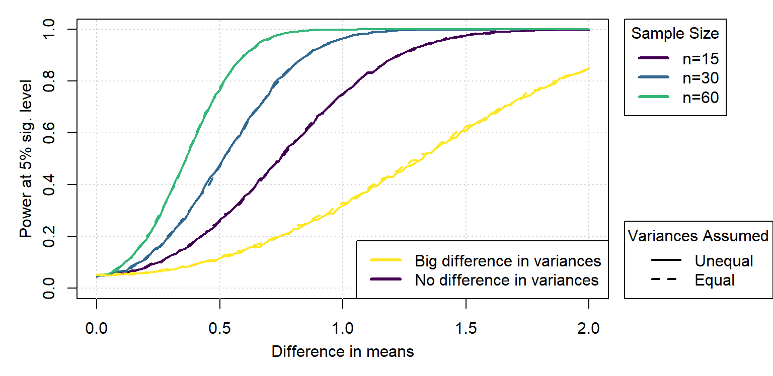
No power is lost when doing the unequal variance test on equal variance data, but accuracy is gained with unequal variances.
It gets worse
If the sample sizes are not the same, specially we double the sample size of the sample with the smallest variance, then we get that the unequal variance test is much better.
Bootstrap test
- A very similar, but more complex argument is made by proponents of a bootstrap version of the t-test.
- They say that you lose little power in the case where the data does meet the t-test assumptions, but gain a lot when it doesn’t.
- Not quite as clear cut though:
- Power loss for small samples is not negligible.
- t-test assumptions usually hold if done right thanks to the Central Limit Theorem and Slutsky’s Theorem.
The data must be normal, Part 1
- Fallacy: the observations must follow a normal distribution in order to do a two sample t-test.
- Truth: it helps if the observations within each group (or residuals) vaguely resemble a normal distribution but is not strictly necessary.
- A t-test assumes that the test statistic follows a t density, but is robust to many kinds of deviations.
- If the data in each sample does actually follow normal distributions then the assumptions are guaranteed to hold.
- If a sample is very skew (e.g. exponential) then it may help to do a transformation first and do the test on the transformed scale, but it needs to be justified (e.g. obvious outliers on a box plot).
The paradox of normality tests
Tests for normality don’t test for normality.
They assume normality and test for evidence to reject it.
- In small samples you often won’t find evidence even if the data structurally can’t be normal.
- In large samples you will usually find evidence, even if the departures from normality are tiny and irrelevant.
- But large samples enjoy the Central Limit Theorem; while small samples are where we really care about the distribution 😒
- This is why so many experts advocate for visual inspection over testing.
If the data is not normal - do a U-test
Another commonly taught rule is that if you reject normality then you should do a Wilcoxon/Mann-Whitney U-test. They call this a non-parametric alternative to the t-test.
However, the U-test has a very different hypothesis, and is thus not an equivalent test.
To quote Wikipedia, the null hypothesis is that …
- “… for randomly selected values X and Y from two populations, the probability of X being greater than Y is equal to the probability of Y being greater than X.”
- It is not that “The medians are equal”, that is an oversimplification that only holds if the two samples are continuous and have the same distribution except for a shift in location. Again people are assuming that the variances are equal.
The non-parametric equivalent to the t-test is the bootstrap t-test.
The p-value tells you about the alternative
Given hypotheses \(H_0\) and \(H_1\), and a test statistic \(S\) with observed value \(s\), we can define a p-value as
\[p=P(S\geq s | H_0)\]
From Bayes’ Theorem we have that
\[P(H_1|s)=\frac{P(s|H_1)P(H_1)}{P(s|H_1)P(H_1)+P(s|H_0)P(H_0)}\]
There is no way to directly relate these quantities, even with extreme assumptions, and yet this is what people love to do.
- There is no obvious practical solution to this impasse, but a good place to start is to never accept any hypothesis. We either fail to reject \(H_0\) and continue to assume that it holds, or we reject \(H_0\) and ?
What are you not showing me?
- If you keep doing tests you will ‘find’ something sooner or later.
- We expect coincidences to pop up 5% of the time even when nothing is happening.
- People keep doing tests and experiments until they find something significant and then try to explain it retroactively.
- They throw out the boring stuff (file-drawer problem)
End result: a lot of published research is not reproducible (over 40% in some psychology journals at one stage).
- Of course this is still miles better than popular media. I’m just saying that there’s room for improvement.
5% is a fine significance level
If you do 100 hypothesis tests (I’ve seen more than 1000 in a single PhD) then the probability of at least 1 false positive is
\[1-\left[(1-0.05)^{100}\right]>99.4\%\]
People are out there talking a lot of nonsense as a result.
Bonferroni said you could decrease your significance level, but I like the Holm-Bonferroni method more, where you inflate your p-values.
- It’s strictly more powerful and just as effective.
- It’s easy to implement, e.g. see ?p.adjust in R.
- Not as powerful as a good multivariate test though - assuming the multivariate assumptions hold 😉
Practical significance
- Practical significance is what really matters.
- Statistical significance should come first, to help avoid analysing coincidences;
- But once you find something statistically significant you have to ask what the practical meaning is.
- The key is the effect size, which is the measure of the practical effect of one thing on another.
- The best effect sizes are so big that anyone can see the impact, and the fancy stats becomes irrelevant!
Regression and Correlation
Manipulating R-square
We start with a proper regression, then we add a noise variable, then we add another 18 noise variables. In theory the regression should get worse right?
set.seed(92340)
x <- rnorm(30)
y <- 2 * x + 30 + rnorm(30)
m <- s <- vector("list", 3)
s[[1]] <- summary(m[[1]] <- lm(y ~ x))

X <- cbind(x, rnorm(30))
s[[2]] <- summary(m[[2]] <- lm(y ~ X))

X <- cbind(X, matrix(rnorm(30 * 18), 30, 18))
s[[3]] <- summary(m[[3]] <- lm(y ~ X))
Results of adding noise to regression
knitr::kable(round(data.frame(R2 = sapply(s, with, r.squared),
    adjR2 = sapply(s, with, adj.r.squared), AIC = sapply(m, AIC),
    BIC = sapply(m, BIC)), 2))
| R2 | adjR2 | AIC | BIC |
|---|---|---|---|
| 0.71 | 0.70 | 92.44 | 96.64 |
| 0.74 | 0.72 | 91.29 | 96.90 |
| 0.96 | 0.87 | 71.20 | 102.03 |
We see \(R^2\) go up a lot. Further, we see \(Adj.R^2\) and AIC improve, with 2 of the noise variables significant at 5%.
The data must be normal, Part 2
- People are super focused on the dependent variable in a regression fitting the assumed distribution (usually normal) but that is not an assumption of regression.
- The observations are assumed to be conditionally normal (or another distribution in the case of a GLM) and if the conditions vary wildly then the observations as a group could have any pattern you can imagine.
- So if the dependent variable isn’t the problem then what is?
- Most issues with regressions are related to the explanatory variables.
- We already know to look out for multicollinearity.
- But lop-sided explanatory variables are also a big problem.
If you have explanatory variables that are very skew (not just a little) then a regression model tends to focus its efforts on the big values, and ignore the nuance in the bulk of the data. In these cases it may help to transform some of them to reduce the skewness and capture more, or just different aspects, of the relationships. Transformations particularly help with correlation analysis.
What was I thinking?
- Most researchers work in such a way that nobody else understands what they are doing most of the time.
- Most researchers coming back to their own work after a short time don’t understand what their own past selves were doing.
- Just think of the average number of revisions on a published paper.
- There is almost always a disconnect between what a researcher thinks, does, and eventually puts down in writing.
The result is that a shocking amount of published research is wrong, or just not reproducible.
Reproducible research
Modern journals of good quality now require that data be published openly (if at all possible) and often that code be published, and published at a high standard at that.
People generally don’t like to have their work questioned, that’s why journals are making these things rules.
The advantages include:
- If anybody can check your work they are much more likely to trust that it’s correct.
- If they disagree with something you did they don’t need to harass you about it, they can just do it their way themselves, and hopefully see why you were right.
And yet, already people are getting so obsessed with these rules that they forget why they were created. Published code helps people follow the details of the methodology, but code is not methodology.
- Just work methodically and it will be easier to make reviewers happy (or slightly less sad).
Conclusion
Thank you for listening
Remember to understand rules and where they come from, don’t just memorise!
- Watch out for the worst tale in statistics: that it’s fine to build your model based on the data and then use that model to judge what relationships are significant based on the model fit to that data.
- If you use observed relationships in the data to build a model for that data then you can’t test those relationships using that model on that data without quickly starting to talk a lot of nonsense.
- You need new data that a model hasn’t seen to test a model. The best way to do that is via controlled experiments where the model is created in advance of collecting the data.