Kurtosis
Source: Wikipedia
We define a function for the sample-size-standardised excess kurtosis.
kurtosis <- function(x) {
  xstand <- x - mean(x)
  kurt <- (sum((xstand)^4))/((sum((xstand)^2))^2)-3/length(x)
  return(kurt)
}
Generate samples
We select random sample sizes and generate a matrix of samples arranged in a list.
We are generating samples from the Stable distribution using the stabledist package.
The index parameter is chosen randomly between 1 and 2. The skewness parameter is set to zero.
n <- 500
minsize <- 20
maxsize <- 1500
samplesizes <- ceiling(runif(n,minsize,maxsize))
alphas <- runif(n,1,2)
library(stabledist)
samples <- mapply(rstable,samplesizes,alphas,rep(0,n))
We used 500 samples of size ranging from 20 to 1500.
Calculate Kurtosis
We use parallel processing to speed up the computation.
library(parallel)
cl <- makeCluster(max(1,floor(0.75*detectCores(logical = FALSE)))) # Select number of cores automatically
nul <- clusterExport(cl,c('kurtosis'))
outputs <- parLapply(cl,samples,kurtosis)
stopCluster(cl)
Graph
We draw a graph of the results.
kurtosis_random <- unlist(outputs)*samplesizes
plot(alphas,kurtosis_random,pch='*',col='black',main='', xlab = expression(alpha), ylab = 'excess kurtosis', log = 'y')
grid()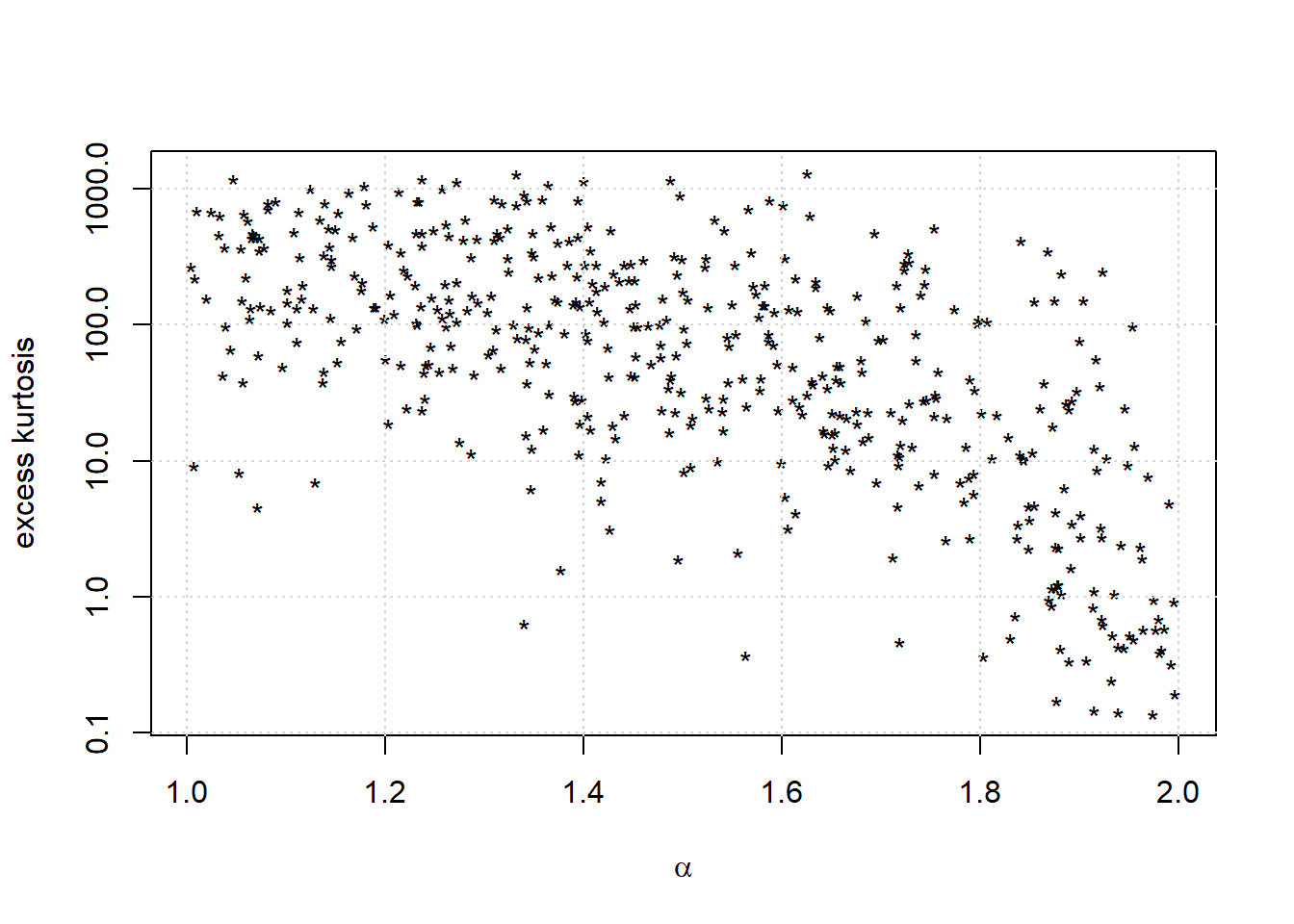
Graph for single sample size
n <- 1000
samplesize <- 500
alphas <- runif(n,1,2)
samples <- sapply(alphas, function(x) {kurtosis(rstable(samplesize,x,0))})*samplesize + 3
plot(alphas,samples,pch=4,col='blue',main=paste('Sample kurtosis for sample size',samplesize), xlab = expression(alpha), ylab = 'Kurtosis', log = 'y')
grid()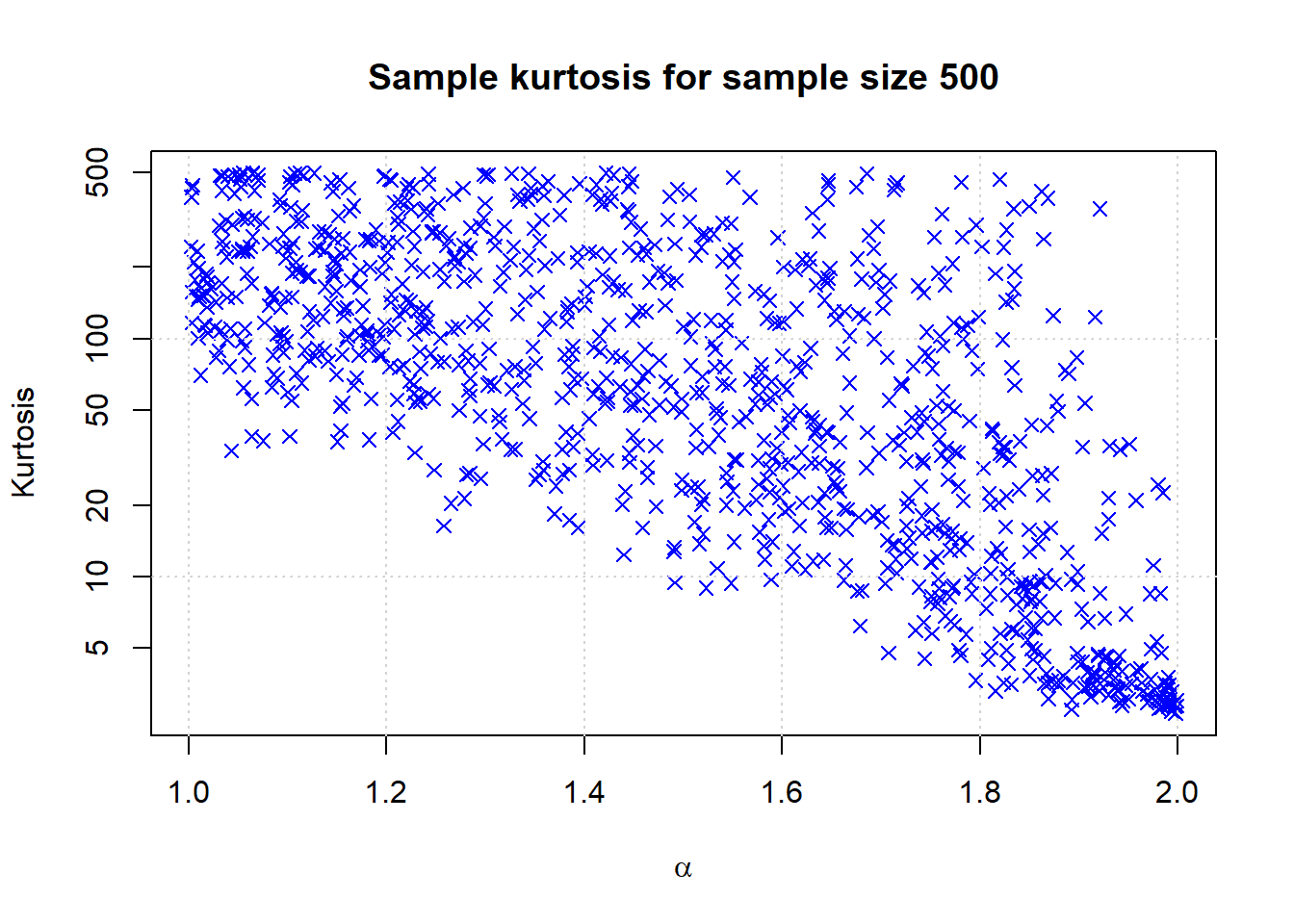
Simulation study
Instead of random values of \(n\) and \(\alpha\), we now use a fixed selection and do a larger scale run.
nsamplespersize <- 25000
minsize <- 50
maxsize <- 500
samplesizes <- seq(minsize,maxsize,minsize)
nsamplesizes <- length(samplesizes)
alphas <- seq(1,2,0.5)
nalphas <- length(alphas)
params <- data.frame(SampleSize=rep(samplesizes,each=nalphas*nsamplespersize),
                     Alpha=rep(alphas,each=nsamplespersize,times=nsamplesizes),
                     Sample=rep(1:nsamplespersize,times=nsamplesizes*nalphas))
samplekurtosis <- function(pars) {
  n <- pars[1]; a <- pars[2]
  x <- rstable(n,a,0)
  xstand <- x - mean(x)
  kurt <- (sum((xstand)^4))/((sum((xstand)^2))^2)-3/n
}
cl <- makeCluster(max(1,floor(0.75*detectCores(logical = FALSE))))
nul <- clusterEvalQ(cl,{suppressPackageStartupMessages(library(stabledist,warn.conflicts=FALSE,quietly=TRUE))})
nul <- clusterExport(cl,c('samplekurtosis'))
outputs <- parRapply(cl,params,samplekurtosis)
stopCluster(cl)
results <- data.frame(params,g_over_n=outputs)
saveRDS(results,file=paste('Kurtosis',gsub(':','_',date()),'.Rds',sep=''))Evaluation of simulation study
library(viridisLite)
cols = viridis(nalphas*2)
g <- results$g_over_n*results$SampleSize
x <- c(0,samplesizes)
tp <- ceiling(0.8*length(samplesizes))
plot(c(0,max(samplesizes)),c(0,max(samplesizes)/2),type='n',xlab = 'Sample size', ylab = 'Excess kurtosis', main='')
grid()
for (a in 1:nalphas) {
al <- alphas[a]
ga <- g[results$Alpha==al]
gg <- results$SampleSize[results$Alpha==al]
ymean <- tapply(ga,gg,mean)
points(samplesizes, ymean, col=cols[a], pch=4)
# lower <- c(0,tapply(ga,gg,quantile,0.05))
# upper <- c(0,tapply(ga,gg,quantile,0.95))
# lines(x, lower, col=cols[a], lwd=1, lty=2)
# lines(x, upper, col=cols[a], lwd=1, lty=2)
lines(x, c(0,ymean), col=cols[a], lwd=2, lty=a)
text(x[tp],ymean[tp],bquote(alpha==.(al)),col=cols[a],pos=3, offset = (a-1)/nalphas)
print(coef(lm(ymean~samplesizes)))
}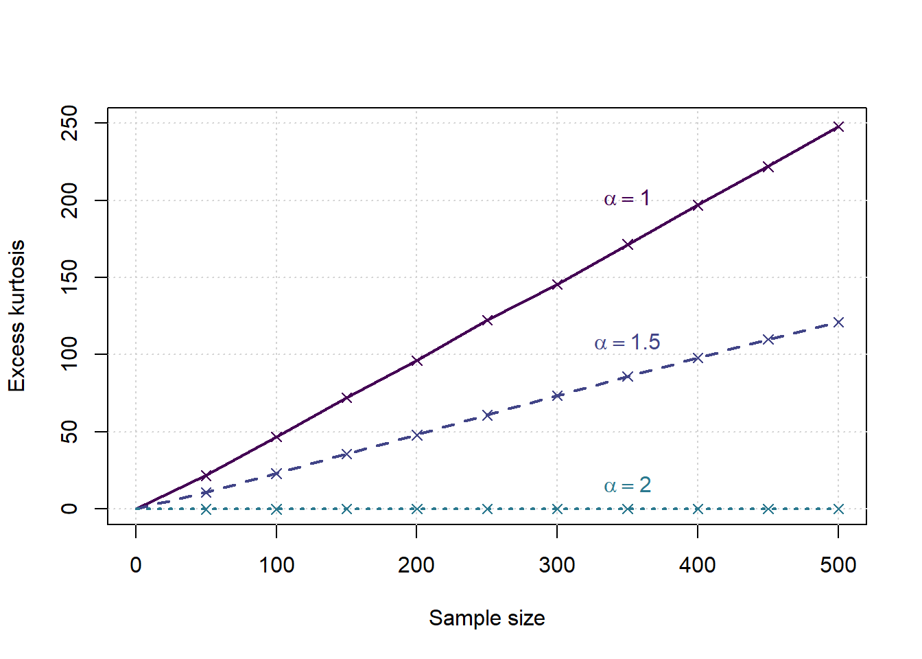
## (Intercept) samplesizes
## -3.5022056 0.5012885
## (Intercept) samplesizes
## -1.3721751 0.2474155
## (Intercept) samplesizes
## -0.0825938600 0.0001743067Simulation Study Alternative: t density
nsamplespersize <- 25000
minsize <- 50
maxsize <- 500
samplesizes <- seq(minsize,maxsize,minsize)
nsamplesizes <- length(samplesizes)
dfs <- c(3,4,5)
ndfs <- length(dfs)
params <- data.frame(SampleSize=rep(samplesizes,each=ndfs*nsamplespersize),
DegFreedom=rep(dfs,each=nsamplespersize,times=nsamplesizes),
Sample=rep(1:nsamplespersize,times=nsamplesizes*ndfs))
samplekurtosis_t <- function(pars) {
n <- pars[1]; df <- pars[2]
x <- rt(n,df)
xstand <- x - mean(x)
kurt <- (sum((xstand)^4))/((sum((xstand)^2))^2)-3/n
return(kurt)
}library(parallel)
cl <- makeCluster(max(1,floor(0.75*detectCores(logical = FALSE))))
nul <- clusterExport(cl,c('samplekurtosis_t'))
outputs <- parRapply(cl,params,samplekurtosis_t)
stopCluster(cl)
results <- data.frame(params,g_over_n=outputs)
saveRDS(results,file=paste('Kurtosis_t',gsub(':','_',date()),'.Rds',sep=''))Evaluation of simulation study
We are interested in the distribution of \(g_2/n\) for various values of \(\alpha\) first, assuming it is stable over \(n\).
cols = viridis(ndfs*2)
g <- results$g_over_n*results$SampleSize
x <- c(0,samplesizes)
tp <- ceiling(0.8*length(samplesizes))
plot(c(0,max(samplesizes)),c(0,max(samplesizes)/22),type='n',xlab = 'Sample Size', ylab = 'Excess kurtosis', main='')
grid()
for (a in 1:ndfs) {
al <- dfs[a]
ga <- g[results$DegFreedom==dfs[a]]
gg <- results$SampleSize[results$DegFreedom==dfs[a]]
ymean <- tapply(ga,gg,mean)
points(samplesizes, ymean, col=cols[a], pch=4)
lines(x, c(0,ymean), col=cols[a], lwd=2, lty=a)
text(x[tp],ymean[tp],bquote("v ="~.(al)),col=cols[a],pos=3, offset = (a-1)/ndfs/2)
print(coef(lm(ymean~samplesizes)))
}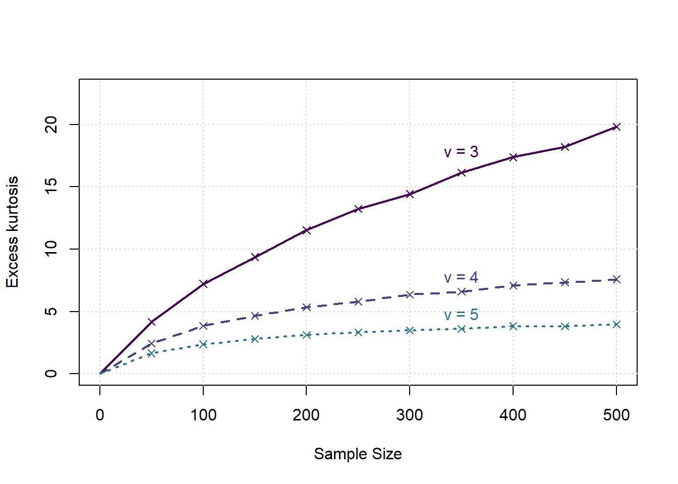
## (Intercept) samplesizes
## 4.05946508 0.03307267
## (Intercept) samplesizes
## 2.80506557 0.01056211
## (Intercept) samplesizes
## 1.936158700 0.004580672Example: Stock Exchange Data
We begin by loading and displaying the New York Stock Exchange index values and related log returns. The data we used is available here.
mydata <- read.csv('nyexchange.csv')
X <- ts(mydata$indexvalue, start = 2013.33, frequency = 251)
lX <- log(X)
lret <- diff(lX)par(mfrow=c(2,1), mar=c(2.2,4.2,1.4,0.2))
cols=viridis(3)
plot(X, main = '', ylab = 'Index value', col=cols[1])
grid()
plot(lret, main='', ylab = 'Log return', col=cols[2])
grid()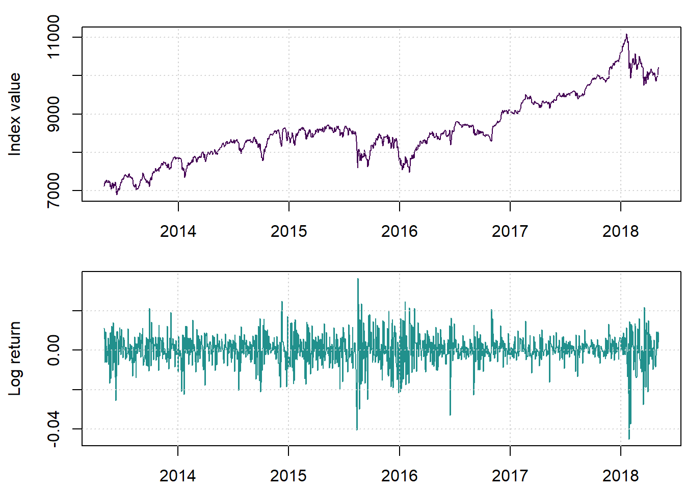
We notice some dramatic movements at places.
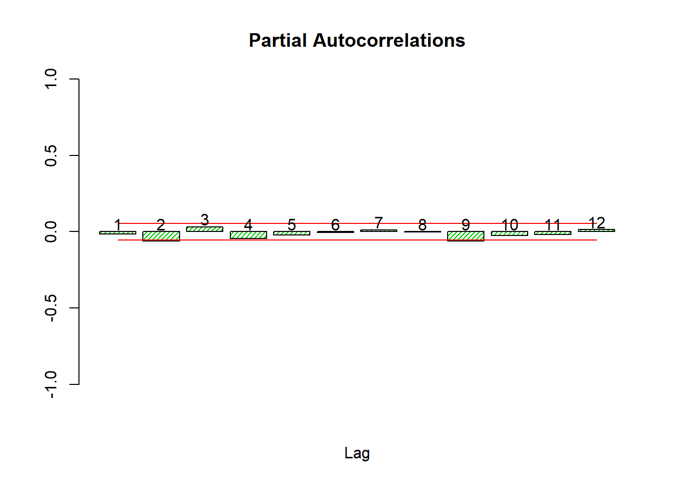
Let’s look at the autocorrelations
source('autocor.r')
autocor(lret)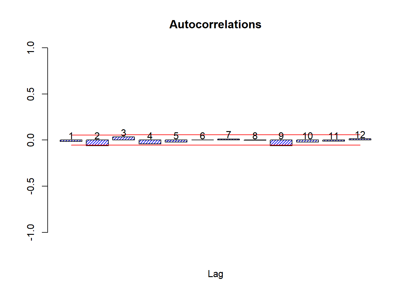
## Autocor Partial Autocor
## [1,] -0.015326596 -0.015326596
## [2,] -0.062281851 -0.062531445
## [3,] 0.033896147 0.032056340
## [4,] -0.040650529 -0.043763370
## [5,] -0.023600168 -0.020789966
## [6,] 0.001727473 -0.005323083
## [7,] 0.012223911 0.012174574
## [8,] -0.001348682 -0.001627343
## [9,] -0.060966241 -0.061690430
## [10,] -0.021055323 -0.024615881
## [11,] -0.011559290 -0.019179503
## [12,] 0.013130875 0.014208423Box.test(lret,24,'Ljung-Box')##
## Box-Ljung test
##
## data: lret
## X-squared = 32.845, df = 24, p-value = 0.1074sqlret <- scale(lret)^2
autocor(sqlret,12)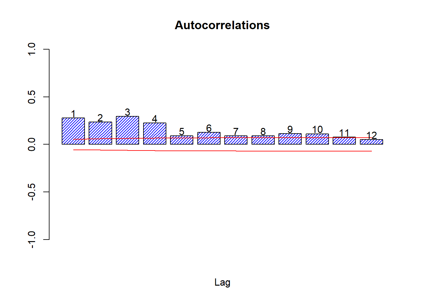
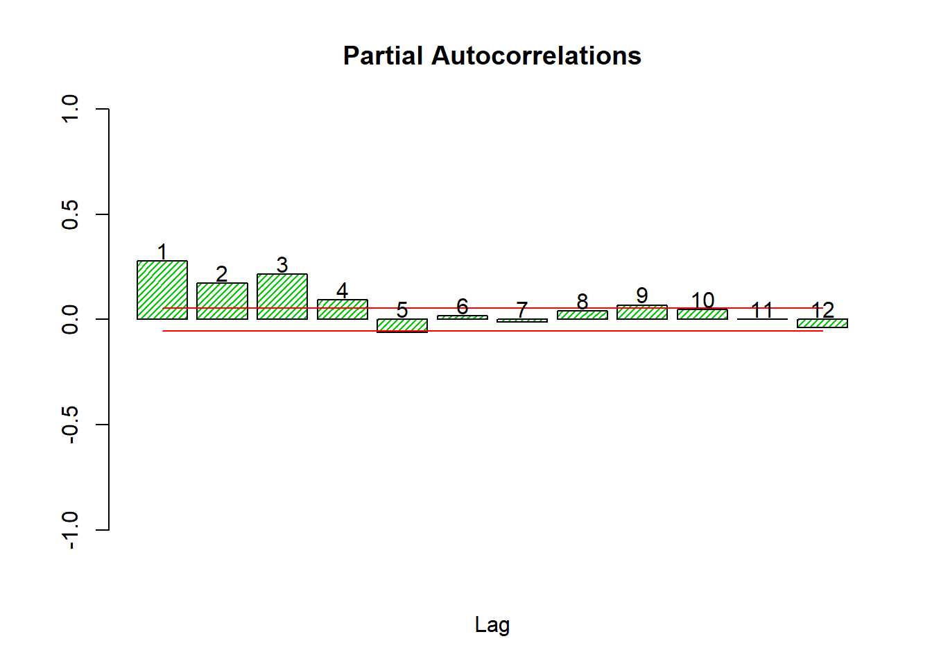
## Autocor Partial Autocor
## [1,] 0.27671624 0.2767162398
## [2,] 0.23497845 0.1715418545
## [3,] 0.29496376 0.2160401858
## [4,] 0.22547585 0.0940220313
## [5,] 0.09085276 -0.0626345435
## [6,] 0.12677680 0.0179938520
## [7,] 0.08865174 -0.0120471599
## [8,] 0.08999092 0.0407826539
## [9,] 0.11403230 0.0680426212
## [10,] 0.11117521 0.0455413827
## [11,] 0.07659700 0.0006617388
## [12,] 0.04947875 -0.0397080496Box.test(sqlret,12,'Ljung-Box')##
## Box-Ljung test
##
## data: sqlret
## X-squared = 434.18, df = 12, p-value < 0.00000000000000022The Box test on the log returns fails to reject white noise for any number of lags from 1 to 36.
The Box test on the squared log returns does reject thoroughly, so we must conclude that autocorrelation exists in the variance only.
For this analysis we are only interested in the data as an uncorrelated sample, so let us consider the histogram instead.
hist(lret, 40, main='', xlab='log return', density = 30, col = cols[1])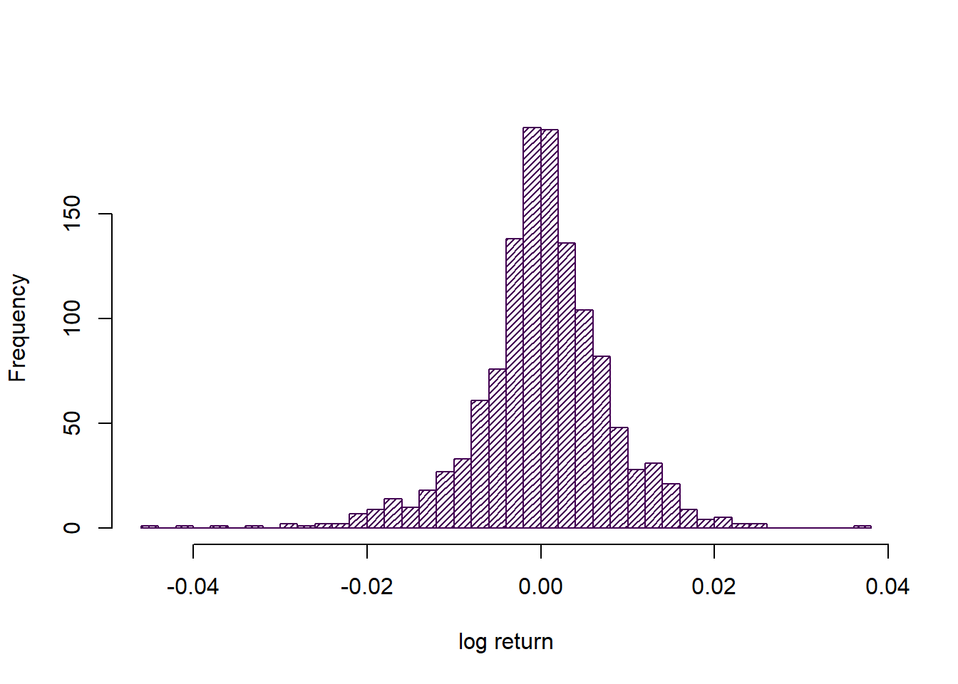
Rolling window calculations
We first calculate kurtosis, then estimates of alpha, for various sizes of rolling window.
library(StableEstim)
print(mainPars <- IGParametersEstim(as.numeric(lret)))## alpha beta gamma delta
## 1.7555602623 -0.3500208698 0.0038817309 0.0005086713T <- length(lret)
ws <- seq(100,500,200)
nws <- length(ws)sta_est_1 <- sta_est_2 <- sta_est_3 <- sta_est_4 <- alphases <- kurts <- skurts <- vector('list',nws)
for (i in 1:nws) {
starts <- 1:(T-ws[i]+1)
skurts[[i]] <- skurt <- sapply(starts, function(x) { kurtosis(lret[x:(x+ws[i]-1)]) } )
kurts[[i]] <- skurt*ws[i]
alphases[[i]] <- (1-skurt)*2
cat('\n\n Starting Kout for window size',ws[i],'\n')
sta_est_4[[i]] <- sapply(starts, function(x) { Estim(EstimMethod='Kout',data=as.numeric(lret[x:(x+ws[i]-1)]))@par[1] } )
cat('Now Kogon-McCulloch \n')
sta_est_1[[i]] <- sapply(starts, function(x) { IGParametersEstim(as.numeric(lret[x:(x+ws[i]-1)]))[1] } )
cat('Now Cgmm\n')
sta_est_3[[i]] <- sapply(starts, function(x) { Estim(EstimMethod='Cgmm',data=as.numeric(lret[x:(x+ws[i]-1)]))@par[1] } )
cat('Now GMM\n')
sta_est_2[[i]] <- sapply(starts, function(x) { Estim(EstimMethod='GMM',data=as.numeric(lret[x:(x+ws[i]-1)]))@par[1] } )
}
windowresults <- list(sta_est_1=sta_est_1, sta_est_2=sta_est_2, sta_est_3=sta_est_3, sta_est_4=sta_est_4, alphases=alphases, kurts=kurts, skurts=skurts)
saveRDS(windowresults,file=paste('NewYorkSErollingWindows',gsub(':','_',date()),'.Rds',sep=''))We considered window sizes of 100, 300, 500.
And plot various things.
plot(c(1,1),c(2,2),type = 'n',xlab = 'Window rightmost point', ylab = 'alpha estimate', main = '', xlim = c(2013.33,(2013.33+T/251)), ylim = c(1.39,2.01))
cols <- viridis(nws*2+1)
for (i in 2) {
w <- ws[i]; st <- w; times <- st:(T-w+st)
lines(2013.33+(times-1)/251,windowresults$alphases[[i]],col=cols[2], lwd=1, lty=(5))
lines(2013.33+(times-1)/251,windowresults$sta_est_1[[i]],col=cols[4], lwd=1, lty=(1))
# lines(2013.33+(times-1)/251,windowresults$sta_est_2[[i]],col=cols[3], lwd=1, lty=3)
# lines(2013.33+(times-1)/251,windowresults$sta_est_3[[i]],col=cols[4], lwd=1, lty=4)
# lines(2013.33+(times-1)/251,windowresults$sta_est_4[[i]],col=cols[5], lwd=1, lty=5)
}
grid()
legend('bottomleft',legend=paste(paste('Window Size',ws[2]),c('Kogon-McCulloch','Kurtosis')),col=cols[c(4,2)],lwd=1,lty=c(1,5))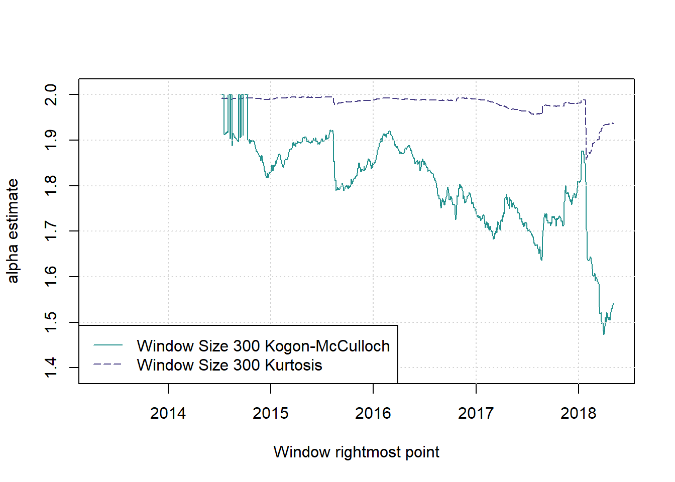
# legend('bottomleft',legend=c(ws,'Kurtosis','Kogon-McCulloch','GMM','Cgmm','Kout'),col=c(cols[1:nws],rep(cols[nws+1],5)),lwd=1,lty=c(rep(1,nws),1:5))
#legend('bottomleft',legend=paste(paste('Window Size',ws),rep(c('Kogon-McCulloch','Kurtosis'),each=nws)),col=cols[c(nws:1,(nws*2):(nws+1))],lwd=1,lty=c(nws:1,(nws*2):(nws+1)))plot(c(1,1),c(2,2),type = 'n',xlab = 'Window rightmost point', ylab = 'Standardised excess kurtosis estimate', main = '', xlim = c(2013.33,(2013.33+T/251)), ylim = c(0,0.25))
cols <- viridis(nws+1)
for (i in 1:nws) {
w <- ws[i]; st <- w; times <- st:(T-w+st)
lines(2013.33+(times-1)/251,windowresults$skurts[[i]],col=cols[nws+1-i], lwd=2, lty=(nws+1-i))
}
grid()
legend('topleft',legend=paste('Window size',ws),col=cols[nws:1],lwd=2,lty=nws:1)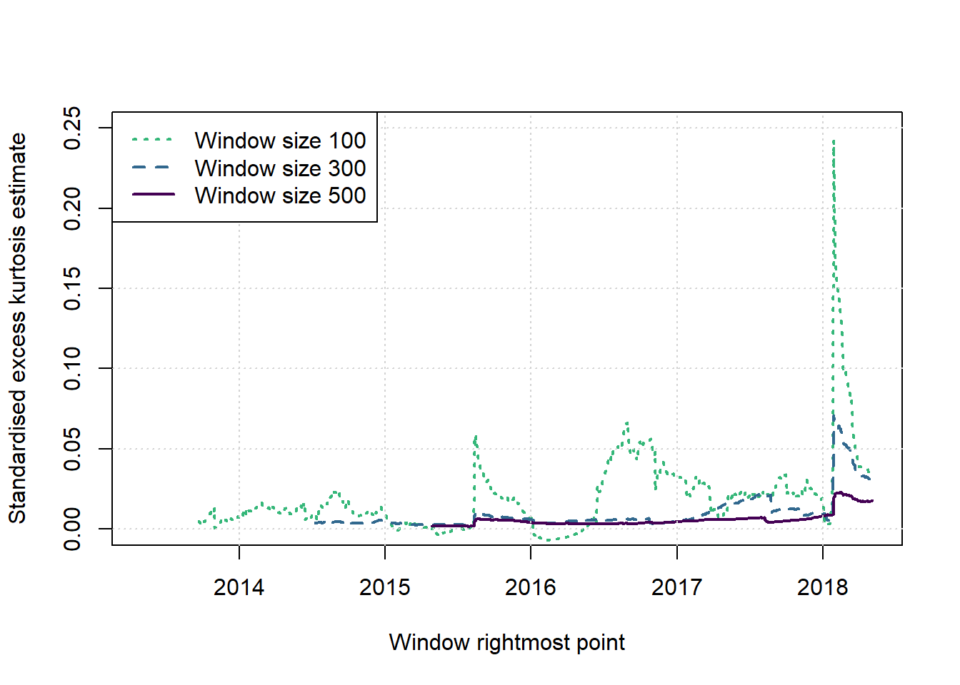
plot(c(1,1),c(2,2),type = 'n',xlab = 'Window rightmost point', ylab = 'kurtosis estimate', main = '', xlim = c(2013.33,(2013.33+T/251)), ylim = c(0,T/50))
cols <- viridis(nws+1)
for (i in 1:nws) {
w <- ws[i]; st <- w; times <- st:(T-w+st)
lines(2013.33+(times-1)/251,windowresults$kurts[[i]],col=cols[nws+1-i], lwd=2, lty=(nws+1-i))
}
grid()
legend('topleft',legend=paste('Window size',ws),col=cols[nws:1],lwd=2,lty=nws:1)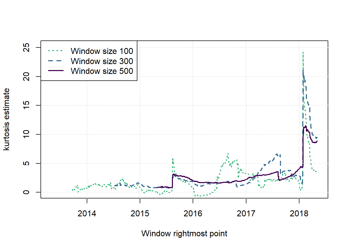
Here we plot the kurtosis using increasing windows, always starting from the first observation and ending at the time on the x-axis.
plot(c(1,1),c(2,2),type = 'n',xlab = 'Date', ylab = 'Excess kurtosis estimate', main = '', xlim = c(2013.33,(2013.33+T/251)), ylim = c(-0.5,4))
cols <- viridis(3)
x2 <- 21:T
kurt <- sapply(x2, function(x) { kurtosis(lret[1:x])*x } )
x <- 2013.33+(x2-1)/251
lines(x,kurt,col=cols[1], lwd=2, lty=1)
grid()
newyorkmdl <- lm(kurt~x)
abline(newyorkmdl, col=cols[2], lwd=1, lty=2)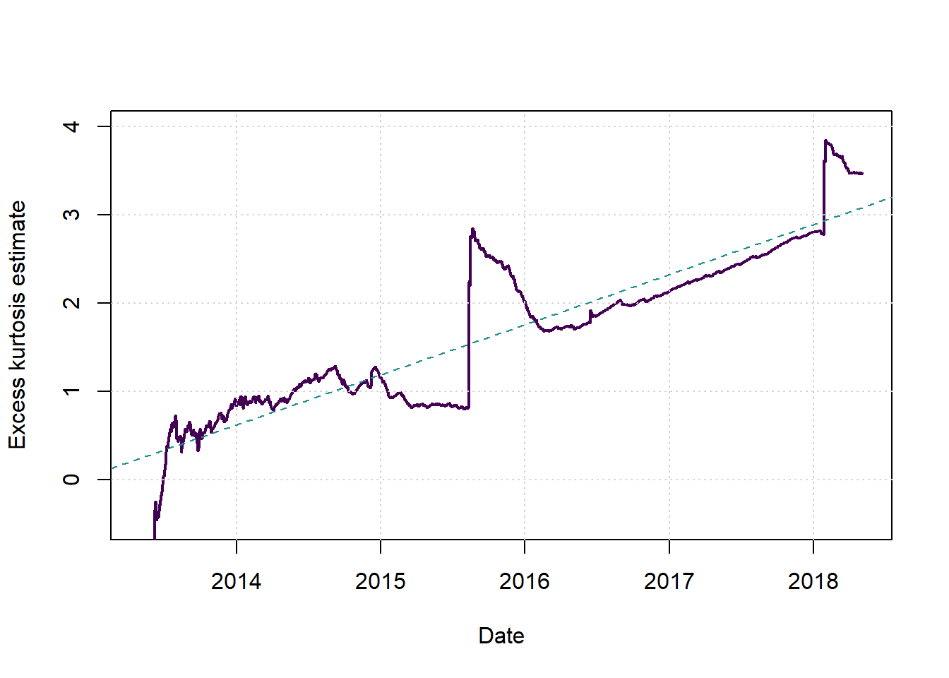
(beta <- coef(lm(kurt~x2))[2])## x2
## 0.002263121(alphaestnewyork <- (1-beta)*2)## x2
## 1.995474Many alphas
ss <- 500
numsmpls <- 5000
alphas <- seq(1,1.95,0.05)
nalphas <- length(alphas)
alphalongvector <- matrix(rep(alphas,each=numsmpls))
samplekurtosisfixed <- function(a) {
x <- rstable(ss,a,0)
xstand <- x - mean(x)
kurt <- (sum((xstand)^4))/((sum((xstand)^2))^2)-3/ss
}cl <- makeCluster(floor(0.75*detectCores(logical = FALSE)))
nul <- clusterEvalQ(cl,{suppressPackageStartupMessages(library(stabledist,warn.conflicts=FALSE,quietly=TRUE))})
nul <- clusterExport(cl,c('samplekurtosisfixed','ss'))
outputs <- parRapply(cl,alphalongvector,samplekurtosisfixed)
stopCluster(cl)
results <- data.frame(alpha=alphalongvector,g_over_n=outputs)
saveRDS(results,file=paste('Kurtosisfixed',gsub(':','_',date()),'.Rds',sep=''))cols <- viridis(5)
ratio <- results[,2]/(2-results[,1])
values <- unlist(tapply(ratio,factor(alphalongvector),mean))
modl2 <- lm(values~alphas)
preds <- predict(modl2,interval = 'confidence')
alldata <- data.frame(ratio=ratio, alpha=alphalongvector)
modl3 <- lm(ratio~alpha, data=alldata)
preds3 <- predict(modl3,newdata=data.frame(ratio=rep(NA,length(alphas)), alpha=alphas),interval = 'confidence')
plot(2-alphas,values,type='p',xlab = expression(2-alpha), ylab = 'Estimated slope', main='', pch=4, col=cols[1],ylim = c(0.4,0.6))
grid()
lines(c(0,1.2),c(0.5,0.5),col=cols[4], lwd=1, lty=1)
lines(2-alphas,preds3[,1], col=cols[2], lwd=1, lty=2)
lines(2-alphas,preds3[,2], col=cols[2], lwd=1, lty=3)
lines(2-alphas,preds3[,3], col=cols[2], lwd=1, lty=3)
legend('topright',legend = c('Means','Proposal','Regression','95% interval'), col=cols[c(1,4,2,2)], lwd = c(NA,1,1,1,1), lty=c(NA,1,2,3,3), pch=c(4,NA,NA,NA,NA))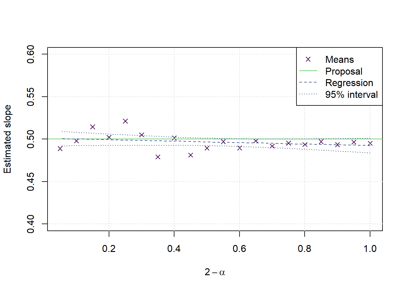
vars <- matrix(0,nalphas,3)
for (a in 1:nalphas) {
currkurt <- results[alphalongvector==alphas[a],2]
currmat <- matrix(currkurt,100)
sds <- apply(currmat,2,sd)
vars[a,1] <- mean(sds)
vars[a,2:3] <- quantile(sds,c(0.05,0.95))
}
plot(c(1,2),c(0,0.4),type='n',xlab = expression(alpha), ylab = 'Standard deviation', main='')
grid()
lines(c(alphas,2),c(vars[,1],0),col=cols[1], lwd=2, lty=1)
lines(c(alphas,2),c(vars[,2],0),col=cols[2], lwd=1, lty=2)
lines(c(alphas,2),c(vars[,3],0),col=cols[2], lwd=1, lty=2)
legend('topright',legend = c('Average SD','90% interval'), col=cols[c(1,2)], lwd = c(2,1), lty=c(1,2))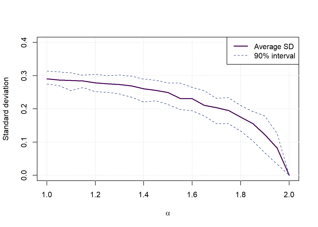
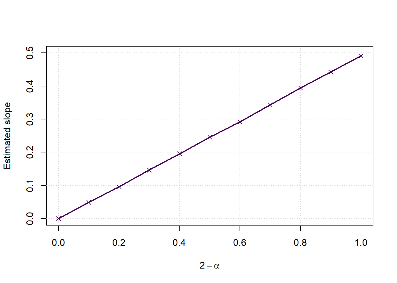
Extending the regression lines to more alpha options
nsamplespersize <- 5000
minsize <- 50
maxsize <- 500
samplesizes <- seq(minsize,maxsize,minsize)
nsamplesizes <- length(samplesizes)
alphas <- seq(1,2,0.1)
nalphas <- length(alphas)
params <- data.frame(SampleSize=rep(samplesizes,each=nalphas*nsamplespersize),
Alpha=rep(alphas,each=nsamplespersize,times=nsamplesizes),
Sample=rep(1:nsamplespersize,times=nsamplesizes*nalphas))
samplekurtosis <- function(pars) {
n <- pars[1]; a <- pars[2]
x <- rstable(n,a,0)
xstand <- x - mean(x)
kurt <- (sum((xstand)^4))/((sum((xstand)^2))^2)-3/n
}library(parallel)
cl <- makeCluster(max(1,floor(0.75*detectCores(logical = FALSE))))
nul <- clusterEvalQ(cl,{suppressPackageStartupMessages(library(stabledist,warn.conflicts=FALSE,quietly=TRUE))})
nul <- clusterExport(cl,c('samplekurtosis'))
outputs <- parRapply(cl,params,samplekurtosis)
stopCluster(cl)
results <- data.frame(params,g_over_n=outputs)
saveRDS(results,file=paste('Kurtosis',gsub(':','_',date()),'.Rds',sep=''))cols = viridis(nalphas*2)
g <- results$g_over_n*results$SampleSize
slopes <- rep(0,nalphas)
for (a in 1:nalphas) {
al <- alphas[a]
ga <- g[results$Alpha==al]
gg <- results$SampleSize[results$Alpha==al]
ymean <- tapply(ga,gg,mean)
slopes[a] <- coef(lm(ymean~samplesizes-1))[1]
}
plot(c(0,1),c(0,0.5),type='n',xlab = expression(2-alpha), ylab = 'Estimated slope', main='')
grid()
points(2-alphas, slopes, col=cols[1], pch=4)
lines(2-alphas, slopes, col=cols[1], lwd=2, lty=1)