29 November 2021

Enjoying this presentation

seanvdm.co.za/presentation

Please open the presentation on your own computer (type link above) to enjoy the following benefits:

  • Exploring the data yourself

  • Interacting with the graphs yourself

  • Moving at your own pace (press o for overview)

  • Maximum quality

    • Try f or F11 for full screen
    • Press w at any time to change to wide screen mode and back
    • Ctrl + Mouse Wheel to zoom

The presentation and source code will be available for download on my website at seanvdm.co.za/files/workshops/mdag2021
Introduction

Abstract

Latent variable models are useful when you have excess observed variables whose values are well explained by a smaller number of underlying, but unobserved, variables. The goal is to simplify the multivariate structure, often to the point where it can be more easily visualised. These models have some similarities to Factor Analysis and Principal Components Analysis, but are parametric models. This presentation discusses an implementation of these models, along with various expansions to handle issues typical of observed data. Expansions discussed include Likert style responses, robust fits, missing value imputation, and possible future directions.

A lot of introductory and supplementary topics are also discussed.

Illustration

Despair

  • Have you faced non-Gaussian data structures (zero inflation / censoring / extremes etc.) with weird dependence relationships (non-linear mixed effects say)?
  • Maybe data on a scale, such as a Likert scale?
  • Do you maybe have multiple response variables? Perhaps too many and a need for dimension reduction?
  • Have you ever looked at the spread of missing values and wanted to cry in despair?
  • What would you do if you encountered ALL of these AT THE SAME TIME?

No need for despair, I’ll show you that you can actually analyse such data in a single unified joint model and answer all the desired statistical questions in a sensible way.

Why Stan?

If all the nuts you ever have to tighten are the same one or two sizes then you buy the best spanners in those sizes. You don’t use a monkey wrench that needs to be set each time. But if you’re encountering different sizes of nuts, fittings, and other objects that need tightening then you get a monkey wrench. In statistical modelling, Stan is the monkey wrench.

According to https://mc-Stan.org/: “Stan is a state-of-the-art platform for statistical modelling and high-performance statistical computation.”

You type out your model in Stan language and then Stan does all the work, including: simulating the whole posterior distribution, simulating the approximate posterior, and/or Maximum Likelihood.

Advantages of Stan

  • It compiles your model into C++ code, so it is very fast
  • Latest simulation methods (HMC+NUTS)
  • Can do usual Bayes, Variational Bayes or Maximum Likelihood as you like - You do not change your model, just one line of code
  • Most importantly, if you want to change your model then you change only the part of the model that needs changing. No changing software, no installing new packages, no changing notation for a different ‘PROC’, etc.

Where Stan might help

Suppose you are doing a regression, but

  • Perhaps a Normal distribution is not appropriate; maybe a t, gamma, GPD, etc. model makes more sense
  • Maybe your observations belong to groups with differing unknown variances
  • Maybe you need to reduce the dimension or work with latent variables
  • Perhaps you have some prior information on one or more parameters
  • Perhaps you have change points, or censoring, or random effects

While tools exist for dealing with each of these issues, each issue has its own tools with their own notations and limitations. Few of these tools can handle any of the other issues at the same time.

With Stan you can handle all these issues at the same time.

Getting help

The Stan language is intuitive and sensible, but you will still need to look up most things the first time you want to use them.

The key bookmark is https://mc-stan.org/users/documentation/ which has everything you need.

I find myself visiting the language functions reference often to see the exact notation for the distribution I want to use.

For the other issues, a standard internet search gets you very far. Stan is popular free software so it has a large and active user base ready to help.

There are many helper packages that can do a lot of (or all) the work for you, including creating the model code for you to play with.

Running Stan

Interfaces

Stan is currently available for R, Python, and C++ as far as I can tell, with other platforms being able to call it via one of those three. We will focus on rstan as it’s the easiest for most statisticians.

There are many ways to use Stan in R:

  • You can type your Stan model in a separate file, then tell rstan to compile that file
  • You can type your Stan model in a Stan block in your R Markdown document and click the play button to compile it
  • You can save the compiled model in a .Rds or Rdata file and then load the compiled model each time you need it
  • You can mix and match the above as it suits you

R Markdown interface

I will use R Markdown to demonstrate.

I use R Markdown for almost everything, including teaching, assessment, consultation, some research, websites, and even making presentations like this one.

To use R Markdown you open RStudio, click File -> New File -> R Markdown…

To put in a Stan model you click on the Insert button at the top right of the code window, then click Stan.

On the next slide I’ll show a very basic Stan model in RStudio.

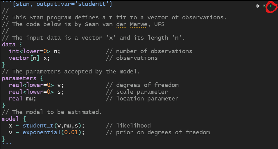
First model: t density

Notice the play button in the top right corner (circled in red).

Model breakdown

The critical components are:

  1. The data
  2. The parameters
  3. The likelihood

The optional components are:

  • Priors for some or all parameters - default is uniform on the domain of the parameter
  • Transformed Parameters - for when your model gets complicated
  • Transformed Data - better to do in R in advance
  • Generated Quantities - for creating things you want later

Installation and Loading

To be able to use rstan the way I do:

  1. Install R
  2. Install Rtools (only needed on Windows, get it where you get R)
  3. Install RStudio
  4. In the RStudio Console window, type install.packages(‘rstan’)
  5. In your code, type library(rstan)

Number of cores

  • Optionally, set the number of cores for Stan to use when simulating in parallel
  • Easiest is to pick a number: options(mc.cores = 3)
  • On most computers you can get a big speed increase easily if you match the number of cores and chains
  • So calculate and store a good number: library(parallel); mycores <- ceiling(0.75*detectCores(logical = FALSE))
  • Then use that number everywhere: options(mc.cores = mycores) and later on when simulating set chains = mycores
  • I like 75% because then I can still use my computer while simulating (i.e. watch YouTube while I’m technically working).

Log returns

Let’s apply the t model to some data.

library(openxlsx)
sourcedata <- read.xlsx("IBM19891998.xlsx")
lret <- sourcedata$LogReturns
dates <- sourcedata$year + sourcedata$month/12 + sourcedata$day/365

cols <- viridisLite::viridis(3)
par(mfrow = c(2, 1), mar = c(4, 4, 2, 0.2))
plot(dates, lret, type = "l", col = cols[1], lwd = 1, xlab = "Date", 
    ylab = "Log return", main = "IBM")
hist(lret, 50, col = cols[2], density = 20, ylab = "Frequency", 
    xlab = "Log return", main = "IBM")

IBM data

Fitting the model

stan_data <- list(x = lret, n = length(lret))  # Create the data list

# Maximum Likelihood / Posterior Mode estimation:
fitML1 <- optimizing(studentt, stan_data)

# This is the main simulation function:
fitBayes1 <- sampling(studentt, stan_data, chains = mycores)
# Type ?sampling for a lot of additional options

saveRDS(fitBayes1, "studenttIBM.Rds")  # Save model fit

summary(fitBayes1)$summary  # See results of simulation

traceplot(fitBayes1)  # See simulation paths to check for stability

list_of_draws1 <- extract(fitBayes1)  # Extract simulations

t model summary

mean se_mean sd 2.5% 97.5% Rhat
v 4.263 0.01 0.371 3.604 5.067 1.000
s 0.013 0.00 0.000 0.012 0.013 1.002
mu 0.000 0.00 0.000 0.000 0.001 1.000

The Rhat measure should always be close to 1.

Rhat compares the variation between chains to the variation within chains, as well as the variation in different parts of each chain. If these are all the same then that is a good indication of convergence in distribution.

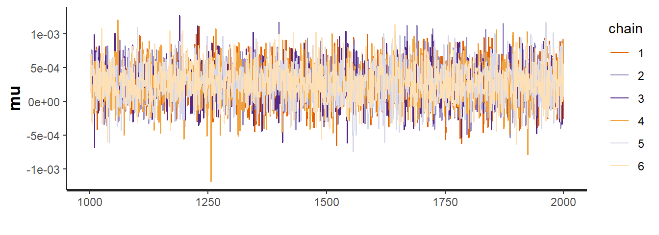
t model trace plot

On the trace plot you should see the same patterns on the left as on the right to indicate that you have done enough burn-in.

You should also see the same sort of patterns in each chain.

When the chains are viewed together they should cover the whole posterior distribution.

Non-standard distributions

We don’t need to only use standard distributions in Stan.

For example, we could use a better prior on the degrees of freedom (provided by Prof Abrie van der Merwe):

\[p(\nu)\propto \left[\psi'(0.5\nu)-\psi'(0.5(\nu+1))-2(\nu+3)\nu^{-1}(\nu+1)^{-2}\right]^{0.5}\]

where \(\psi'\) is the trigamma function.

Working with the results

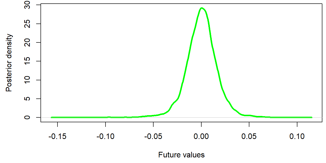
# Posterior Predictive Distribution
postpred1 <- rt(length(list_of_draws1$mu), list_of_draws1$v) * 
    list_of_draws1$s + list_of_draws1$mu
par(mar = c(4.4, 4.4, 0.4, 0.4))
plot(density(postpred1), xlab = "Future values", ylab = "Posterior density", 
    main = "", col = "green", lwd = 3)

Intervals and p-values

After fitting the model, we can obtain intervals for any quantity of interest as follows:

  • Calculate the quantity for each simulated parameter vector, to get a vector of quantities
  • This vector of quantities can be seen as an approximation to the posterior distribution of the quantity of interest, let us call it sims.
  • Calculate a symmetric interval, say 95%, using the built-in quantile function: quantile(sims,c(0.025,0.975))
  • Calculate an equivalent to the traditional two-sided p-value using this function:
pvalfunc <- function(sims, target = 0) {
    2 * min(mean(sims < target), mean(sims > target))
}

Shortest interval

For a given coverage, a shorter interval provides more useful information.

If the distribution of the quantity of interest is skew then the symmetric interval is not ideal.

We can calculate the shortest interval, also known as the highest posterior density (HPD) interval, quite easily though if we have simulations (also works for bootstraps).

The process is simple: to get the shortest 95% interval, just work out the length of every 95% interval and see which one is the shortest!

shortestinterval <- function(sims, alpha = 0.05) {
    # Coded by Sean van der Merwe, UFS
    sorted.sims <- sort(sims)
    nsims <- length(sims)
    gap <- round(nsims * (1 - alpha))
    widths <- diff(sorted.sims, gap)
    interval <- sorted.sims[c(which.min(widths), (which.min(widths) + 
        gap))]
    return(interval)
}

Simulate once, calculate many

Once you have a set of simulations, you can calculate estimates, intervals, and probabilities to your heart’s content:

  1. Assume the first set of simulated parameters are the true values.
  2. Calculate the quantity of interest using those parameters.
  3. Repeat for simulations 2 to … and keep all the answers.
  4. Summarise the vector of answers using mean, summary, quantile, hist, etc.

Example: to calculate \(P[\mu^2>5]\) we type

mean(list_of_draws1$mu^2 > 5)
## [1] 0

Binomial responses

Likert Scale as Binomial

Assume we are measuring something on a scale and we have reason to believe that the underlying process is continuous but forced into the scale at some stage in the data generating process.

Suppose we have Likert scale questions with 5 levels, then we can mark them as 0, 1, 2, 3, and 4.

In the Binomial GLM formulation it is assumed that the responses \(y_i\sim Binomial(4, p_i)\), while \(logit(p_i)=f(\mathbf{x}_i)\) where \(f(\mathbf{x}_i)\) is some function of the explanatory variables corresponding to observation \(i\) (linear function for a true GLM). In the simplest case we have a constant/intercept only: \(f(\mathbf{x}_i)=\beta_0\), but we could just as easily include predictors such as age or gender in this framework.

Generate raw data

Suppose we ask some students whether they have a good lecturer.

set.seed(12345)
n <- 100
Age <- rpois(n, 3) + 18
Gender <- round(runif(n))
Likert <- rbinom(n, 4, plogis(-2 + 0.1 * Age + 0.3 * Gender))

Response by age

All at once

Standard GLM

Here we fit a Binomial GLM to the response in the standard way:

y <- Likert/4
s1 <- coef(summary(glm(y ~ Age + Gender, family = binomial(), 
    weights = rep(4, n))))

Stan GLM

There are several easy ways to do a GLM using Stan. The rstanarm and brms packages are highly recommended as easy interfaces for using Stan and for doing Bayes in general.

However, we are going to do it the hardcore way, for reasons that will make sense later. We will code the model in Stan ourselves.

We will use the the STAN interface via rstan to implement our models.

library(parallel)
library(rstan)
mycores <- max(1, floor(detectCores(logical = FALSE) * 0.75))
options(mc.cores = mycores)
rstan_options(auto_write = TRUE)

Model definition

data {
  int<lower=2> n;            // number of observations
  int<lower=1> m;            // maximum value of observations
  int<lower=0, upper=m> y[n]; // observations
  int<lower=1> k;            // number of explanatory variables, including intercept
  row_vector[k] x[n];            // explanatory matrix
}
parameters {
  vector[k] beta;            // coefficients
}
model {
  for (i in 1:n) {
    y[i] ~ binomial_logit(m, x[i]*beta);
  }
}

Simulation results

BinResults <- sampling(Binomial1, list(n = n, m = 4, y = Likert, 
    k = 3, x = model.matrix(~Age + Gender)), chains = mycores)
# plot(BinResults)
BinResSims <- extract(BinResults)

Simulation results visual

Pause, ponder, and question

  • How could your work be improved with access to a modelling tool with such flexibility?
  • What would be the obstacles to using this?

PCA

Generate raw data

In this example we are first going to take some multivariate normal data and apply PCA to it.

library(MASS)
set.seed(12345)
under_Dim <- 2
full_Dim <- 5
true_weights <- matrix(runif(full_Dim * under_Dim, -3, 3), 
    under_Dim, full_Dim)
n <- 100
rawZ <- mvrnorm(n, rep(0, under_Dim), diag(rep(1, under_Dim)))
rawX <- matrix(rnorm(n * full_Dim), n, full_Dim) + rawZ %*% 
    true_weights
GroupNum <- (rowSums(rawZ) > 0) + 1
Group <- c("🐬", "🐪")[GroupNum]

We are using 2 underlying dimensions and random weights to relate those dimensions to the 5 observed dimensions.

For fun, we create a grouping variable based on whether the underlying variables are positive on average and see whether we can see the separation later.

Visualising the raw data

Our raw data has 6 dimensions, which makes it a challenge to visualise. We can try though. In this case I used a logistic transform of the 5th variable for size, and you have to mouse over to see the group. It is not easy to see the multivariate structure.

Scale data

It is often a good idea to scale the data, although not always. We do so here, but not in all cases going forward.

X <- scale(rawX)
round(colMeans(rawX), 4)
## [1]  0.3660  0.5959 -0.4640  0.1253  0.6005
round(colMeans(X), 4)
## [1] 0 0 0 0 0

The means are now zero and the standard deviations one.

  • Random side note: if you are running my code on your computer then replace the emojis with the usual ‘Group A’ and ‘Group B’ before knitting.

Standard PCA

Bayesian Latent Variable Model

// This Stan block defines a basic Bayesian PCA, Joseph H. Sakaya & Suleiman A. Khan
// https://www.cs.helsinki.fi/u/sakaya/tutorial/code/pca.R 
data {
    int<lower=0> N;    // Number of samples
    int<lower=0> D;    // The original dimension
    int<lower=0> K;    // The maximum latent dimension, must be < D
    matrix[N, D] X;   }// The data matrix
parameters {
    matrix[N, K] Z;    // The latent matrix
    matrix[D, K] W;    // The weight matrix
    real<lower=0> tau; // Noise term 
    vector<lower=0>[K] alpha; } // ARD prior
transformed parameters{
    vector<lower=0>[K] t_alpha;
    real<lower=0> t_tau;
  t_alpha = inv(sqrt(alpha));
  t_tau = inv(sqrt(tau)); }
model {
    tau ~ gamma(1,1);           
    to_vector(Z) ~ normal(0,1);
    alpha ~ gamma(1e-3,1e-3);               
    for(k in 1:K) W[,k] ~ normal(0, t_alpha[k]);
    to_vector(X) ~ normal(to_vector(Z*W'), t_tau); }

. . . . . . . . . . . . . . . . . See https://www.cs.helsinki.fi/u/sakaya/tutorial/ for more info.

Simulation and processing

reduced_Dim <- full_Dim - 1
stan_data <- list(N = nrow(X), D = ncol(X), K = reduced_Dim, 
    X = X)
modelfit <- sampling(PCAbasic1, stan_data, pars = c("alpha", 
    "tau", "W", "Z"), iter = 4000, chains = mycores)
# modelfit <- vb(PCAbasic1, stan_data, pars=c('alpha',
# 'tau', 'W', 'Z')) # , algorithm = 'fullrank')
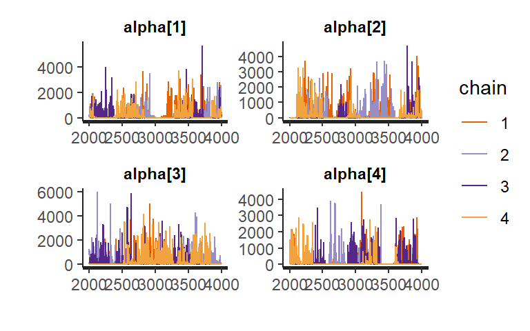
traceplot(modelfit, c("alpha"))

sims <- extract(modelfit)

The non-identifyability problem

  • In a regular PCA the latent dimensions are not naturally in the ideal order, they are sorted after calculation according to the eigenvalues. Similarly, we must sort the latent dimensions here.

  • However, as can be seen on the trace plot, the latent dimension order is constantly changing across simulations.

  • The full posterior distribution includes all possible orderings of the latent dimensions. 😲

    • People use variational inference to fit the model instead of simulations, often arriving at only a single ordering; but it doesn’t fully solve the problem.
    • Variational inference can be much faster in large samples though, where it also the most accurate. Stan does variational inference in a very clever way.
  • The latent dimensions can also be flipped arbitrarily, and are in the simulations.

Dimension order

Here we sort each simulation vector by the order of the weight of the dimensions.

nsims <- length(sims$tau)
orders <- apply(sims$alpha, 1, order)
for (sim in seq_len(nsims)) {
    sims$W[sim, , ] <- sims$W[sim, , orders[, sim]]
    sims$Z[sim, , ] <- sims$Z[sim, , orders[, sim]]
    sims$alpha[sim, ] <- sims$alpha[sim, orders[, sim]]
}

At this stage the weights per dimension are almost perfectly bimodal. Consider the weight of the first variable in the first dimension:

Dimension orientation

So we pick a direction for each dimension and flip dimensions as needed per simulation.

In this case we use the direction of the first variable as the anchor, but this can be changed, or done multiple times for different anchors to be sure.

anchor <- 1
for (dim in seq_len(reduced_Dim)) {
    flip <- sims$W[, anchor, dim] < 0
    sims$W[flip, , dim] <- -sims$W[flip, , dim]
    sims$Z[flip, , dim] <- -sims$Z[flip, , dim]
}

Proportions of variation explained

Once the dimensions are sorted we can calculate the proportion of variation explained by each dimension.

MedianVariation <- apply(1/(sims$alpha), 2, median)
PoV_Bayes <- MedianVariation/(sum(MedianVariation) + median(1/sims$tau))

The cumulative proportion of variation explained by the model is theoretically 65.7, 21.7, 2.5, 0.4.

The proportion of variance explained by the model, calculated for each variable and averaged, is practically 69.1, 5.4.

The reason why we resort to this alternative calculation will become clearer soon.

Latent variable model results

More rotation

Pause, ponder, and question

  • Why go through all this trouble to get essentially the same results as we got from the simple PCA?

Combining

Now for the magic

Now for the magic: what if I had multiple Likert scale responses and wanted to do a PCA style analysis?

LikertScale <- c("Strongly Disagree", "Disagree", "Neutral", 
    "Agree", "Strongly Agree")
nLikert <- length(LikertScale)
set.seed(12345)
Y <- plogis(rawZ %*% true_weights)
Y <- matrix(rbinom(length(Y), nLikert - 1, Y), nrow(X), 
    ncol(X))

Multiple responses visual

Multiple Likert Scale Responses Model

// This Stan block defines a Bayesian PCA, Joseph H. Sakaya & Suleiman A. Khan but
// with the dependent variable changed to Binomial (by Sean van der Merwe, UFS)
data {
    int<lower=0> N; // Number of samples
    int<lower=0> D; // The original dimension
    int<lower=0> K; // The maximum latent dimension, must be < D
    int<lower=0> M; // The binomial maximum
    int<lower=0, upper=M> X[N*D]; // The data matrix as vector
}
parameters {
    matrix[N, K] Z; // The latent matrix
    matrix[D, K] W; // The weight matrix
    vector<lower=0>[K] alpha; // ARD prior
}
transformed parameters{
    vector<lower=0>[K] t_alpha;
  t_alpha = inv(sqrt(alpha));
}
model {
    to_vector(Z) ~ normal(0,1);
    alpha ~ gamma(1e-3,1e-3);               
    for(k in 1:K) W[,k] ~ normal(0, t_alpha[k]);
    X ~ binomial_logit(M, to_vector(Z*W'));
}

Proportion of variation

We calculate the proportion of variation in a crude way, by looking at the square differences of predicted and observed values.

We do this for 0, 1, and 2 dimensions and combine the numbers to get the marginal variation explained.

ScaleMax <- 4
varhat <- sd(stan_data$X)^2
Zhat <- apply(sims$Z, 2:3, median)
What <- apply(sims$W, 2:3, median)
varhat1 <- sd((plogis(c(Zhat[, 1] %*% t(What[, 1]))) * ScaleMax) - 
    stan_data$X)^2
varhat2 <- sd((plogis(c(Zhat[, 1:2] %*% t(What[, 1:2]))) * 
    ScaleMax) - stan_data$X)^2
(PoV_Bayes <- c(varhat - varhat1, varhat1 - varhat2)/varhat)
## [1] 0.74633945 0.05618205

Multiple Likert Scale Responses Results

Missing values

What if some of the values were missing (MCAR)?

nMissing <- 50
nTotal <- stan_data$N * stan_data$D
whichMissing <- sample.int(nTotal, nMissing)
Y2 <- Y
Y2[whichMissing] <- NA_integer_
whichObs <- seq_len(nTotal)[-whichMissing]

Missing data model

// This Stan block defines a Bayesian PCA, Joseph H. Sakaya & Suleiman A. Khan but with the dependent variable changed to Binomial and missing values added by Sean  van der Merwe, UFS
data {
    int<lower=0> N; // Number of samples
    int<lower=0> D; // The original dimension
    int<lower=0> K; // The maximum latent dimension, must be < D
    int<lower=0> M; // The binomial maximum
    int<lower = 0> N_obs; // Total number of observed values in matrix
    int<lower=0, upper=M> X[N_obs]; // The data matrix as vector, only observed
    int<lower = 1, upper = N*D> ii_obs[N_obs]; }
  // Indicator vector of which values are observed in the matrix (column wise)
parameters {
    matrix[N, K] Z; // The latent matrix
    matrix[D, K] W; // The weight matrix
    vector<lower=0>[K] alpha; }// ARD prior
transformed parameters {
    vector<lower=0>[K] t_alpha;
    vector[N*D] zw;
  t_alpha = inv(sqrt(alpha));
  zw = to_vector(Z*W'); }
model {
    to_vector(Z) ~ normal(0,1);
    alpha ~ gamma(1e-3,1e-3);               
    for (k in 1:K) W[,k] ~ normal(0, t_alpha[k]);
    X ~ binomial_logit(M, zw[ii_obs]); }

Missing data model fit

stan_data <- list(N = nrow(Y2), D = ncol(Y2), K = 4, X = c(Y2)[whichObs], 
    M = 4, N_obs = (nTotal - nMissing), ii_obs = whichObs)
binfit <- sampling(PCAbinomialMissing, stan_data, pars = c("alpha", 
    "W", "Z"), iter = 4000, chains = mycores)
varhat <- sd(stan_data$X)^2
Zhat <- apply(sims$Z, 2:3, median)
What <- apply(sims$W, 2:3, median)
varhat1 <- sd((plogis(c(Zhat[, 1] %*% t(What[, 1]))) * ScaleMax)[whichObs] - 
    stan_data$X)^2
varhat2 <- sd((plogis(c(Zhat[, 1:2] %*% t(What[, 1:2]))) * 
    ScaleMax)[whichObs] - stan_data$X)^2
PoV_Bayes <- c(varhat - varhat1, varhat1 - varhat2)/varhat

Missing data model results

Missing values

The model is fitted using all of the observed values and none of the missing values. This is an ideal approach for data Missing Completely at Random (MCAR).

In the case of Missing at Random (MAR) and even Missing Not at Random (MNAR) where the missingness mechanism is based on the latent values, this approach is still probably a great approach, although I haven’t tested it. For really complicated missingness, it may be possible to expand the models discussed to include additional external information, but this is beyond the scope of today’s presentation.

These models all naturally produce uncertain predictions of the missing values in the data set as a by-product, so multiple imputation is a breeze:

nImpute <- 10  # Number of new data sets to impute
SimsSelection <- sample(seq_len(nsims), nImpute)  # Pick random set of simulations
NewDataSets <- lapply(SimsSelection, function(sim) {
    preddata <- rbinom(n * full_Dim, ScaleMax, plogis(c(sims$Z[sim, 
        , ] %*% t(sims$W[sim, , ]))))  # Predict all values
    preddata[whichObs] <- stan_data$X  # Put back values we know for sure
    preddata <- matrix(preddata, n)  # Put it in columns
    preddata  # Return the filled in data set
})
# Write all data sets to an Excel file with each data
# set on a sheet
openxlsx::write.xlsx(NewDataSets, "ImputedData.xlsx")

Pause, ponder, question

Let us pause here a moment and think about what we have discussed.

  • We have an algorithm that can easily produce a joint predictive posterior distribution over all observations, including missing values, regardless of the apparent marginal distributions.

    • Multiple imputation of any number of plausible datasets is thus a breeze.
  • The only major assumption is the existence of an underlying latent structure of lower dimension that explains the observed variation via linear transformation.

Over the top fun time

Let us go nuts with distributions

What if the first variable was normal, but then the second one had some extreme values, so maybe a \(t\) density would fit better? What if the third variable was something counted, so maybe a Poisson distribution? The fourth variable can be a True/False question and the last one a Likert scale.

Let’s do a latent variable analysis and see if we can still get the underlying latent dimensions out of the chaos. 😀

Chaos results

Moooorrreee Poowwwweeerrrr!!!!

We’re going to stop the crazy here, but some things you could try at home:

  • Bring in structure to the underlying latent dimensions
  • Test whether the dimensions are related to an external factor
  • Predict new or other things using the latent dimensions

The uncertainty problem

So far we just took means

The plots are done on a best guess basis; so there are many kinds of uncertainty we are ignoring, such as:

  • The latent values are not certain (in any dimension)
  • The relative orientation of the variables is not certain
  • The absolute orientations of the variables are not certain
  • The distributions are not certain
  • The simulation accuracy is not certain
  • The weights are not certain
  • The relevant dimensions are not certain
  • The order of the dimensions is not certain
  • The missing values are not certain

Incorporating half of the uncertainty

If we give each point a rectangle indicating the shortest 50% interval in each dimension then we get a lot of uncertainty

Some uncertainty doesn’t matter

  • The uncertainty in the dimension weights and orders are usually small relative to those weights, so the preferred order of at least the first few dimensions is usually quite clear

  • The relevant dimensions can be chosen by practicality (say 2 for a presentation like this one)

    • You can also do a scree plot, but with the bonus that you could add confidence limits to the plot if you wanted to
  • The distributions have little impact as long as they are chosen sensibly

    • Like using Negative Binomial instead of Poisson if you have over-dispersion
  • The simulation accuracy is reported by Stan and if it is too large you can just do more simulations

Orientation

We’ve already looked at flipping the dimensions using a variable as an anchor.

We can go further and also rotate and scale the plot using a single anchor, to further reduce the arbitrary uncertainty that doesn’t matter.

Z <- Csims$Z[, , 1:2]
W <- Csims$W[, , 1:2]
anchorPoint <- colMeans(W[, 1, ])
anchorAngle <- atan(anchorPoint[2]/anchorPoint[1])
for (sim in 2:nsims) {
    currentAngle <- atan(W[sim, 1, 2]/W[sim, 1, 1])
    rotMat <- matrix(c(cos(anchorAngle - currentAngle), 
        -sin(anchorAngle - currentAngle), sin(anchorAngle - 
            currentAngle), cos(anchorAngle - currentAngle)), 
        2)
    W[sim, , ] <- W[sim, , ] %*% rotMat
    Z[sim, , ] <- Z[sim, , ] %*% rotMat
    currentPoint <- W[sim, 1, 1]
    W[sim, , ] <- W[sim, , ] * anchorPoint[1]/currentPoint
    Z[sim, , ] <- Z[sim, , ] * anchorPoint[1]/currentPoint
}

Uncertainty in variables

Let us look at the angles of variables 1 and 2 across simulations before and after this transformation:

Fuzzy latent points again

Perhaps now the remaining uncertainty in the points might be easier to visualise, or perhaps the inherent uncertainty in trying to estimate what we cannot directly observe is just that large?

  • It seems that over-analysing a biplot is a quick road to spurious results.

Conclusion

Thank you for listening

  • Stan is the flexible all-purpose solution for people who find themselves with unusual statistical modelling problems.

  • It can do much more advanced stuff than what was shown here. See their website for more information.

  • The help files are extensive. The reference documents are the most useful when you are trying to solve a specific problem.

  • There are many helper packages that can do a lot of the work for you, including creating basic model code.

    • The models you saw today were created manually though.
  • Fitting models with Stan can be a lot of fun because of the freedom it provides.