Simulation is fun

Sean van der Merwe

Introduction

With simulated data you know the right answers up front. Real data has issues. Simulated data that looks and sounds like real data is the best, both for assignments and for research.

Outline

Me
More about me
My passions
Simulating data for assignments

Me

Thank you for the invitation to talk about me, it’s my favourite topic.

History

I’ve been on the UFS campus in various capacities for over 4 decades
Started formally lecturing full time in 2006
Taught over a dozen different modules in a short space of time
- Exciting, interesting, enlightening, but not ‘productive’
- The research focussed idea of productivity and success is mostly wrong, but it is reality (in spite of policy)
- I was stubbornly teaching focussed, but it gradually changed from focussed to just stubborn
So end of 2018 I made the switch to consultation as my primary focus
- Went from 2 projects/year to 40+ projects/year (max. 60)

Consultation is fun

I do consultation within the UFS for all sorts of things (not just stats)
- I was the designated statistician on two ethics committees for the last 6 years
  - Research ethics really helps you to see the fundamentals of research, and also its breadth and impact
I’ve worked with people from every faculty
I’ve helped on every level from the Rector down
The best is the people doing clean science where it is obvious what to do, but the more fuzzy problems can get you excited too
I highly recommend consultation to everyone

No, like really, for everyone

When you talk to non-statisticians about statistics you have to bring across the core concepts efficiently and effectively
- This forces you to think through and deeply understand the core concepts
Real data has issues, forcing you to broaden your mind and skills
- Bubbles, silos and echo-chambers exist in statistics
Builds perspective: you learn quickly what are the concepts that really matter, and which don’t (or no longer)

Research, consultation, and research consultation all make you a better lecturer!

More about me

Bayes is great

I love using Bayes whenever a problem gets interesting or ‘interesting’
Once you’ve simulated from the posterior you can calculate anything you want easily
Prediction with uncertainty is straightforward, even for really complicated models
- Or combinations of models
Bayes research typically involves a lot of simulations, which is my real speciality

Current research projects

Improved estimation of a skewed Student distribution and robust regression on the conditional mode
Addressing outliers in mixed-effects logistic regression: a more robust modelling approach
An improved outlier- and skewness-robust framework for quantile regression models
Joint quantile regression of longitudinal continuous proportions and time-to-event data: application in medication adherence and persistence
Prior selection for estimating the number of missing extreme values
Harnessing Bayesian Modelling for Enhanced Decision-Making in Group Insurance Pricing

Supervision

Between 0 and 7 PhD students on any given day (+1M, +1H)
depending on whether you count the ones who are registered but vanished, the ones claiming to be ‘working on it’, the one who is present but not registered yet, and the ones who I help even though they aren’t my students
I try to help them not repeat my mistakes, but they keep doing it
- Mistakes like not spending enough time on literature
- Being too focussed on teaching/work, not realising that research skills are transferable and being more efficient at both teaching and research is a virtue worth cultivating
- Obsessing over each project instead of publishing imperfect work and moving on

Basics of simulating

Simulating from distributions

Hit refresh (F5 or Ctrl+r) if nothing is showing.

Simulating categorical data

Example: Let’s shuffle a deck of cards

deck <- paste( c(2:10, 'Jack', 'Queen', 'King', 'Ace') |> rep(times=4), 'of',
               c('Spades','Diamonds','Clubs','Hearts') |> rep(each=13) )
# To draw a hand of 7 cards:
hand <- deck |> sample(7)

# Shuffling is taking a sample the same size (52) without replacement:
shuffled_deck <- deck |> sample(length(deck))

# To do a bootstrap sample just add: , TRUE

Generate and save

n <- 100
data.frame(
  Mark = rbinom(n, 100, 0.6), 
  Group = c('🐬', '🐪') |> sample(n, replace = TRUE), 
  Height = rnorm(n, 1.67, 0.1)
) |> openxlsx::write.xlsx('gen_data_1.xlsx')

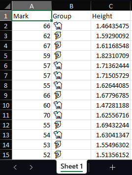
Writing to Excel nicely

You might think, “Let me make it look nice manually by opening it in Excel,” but they you decide to generate new data and you have to repeat those steps, again and again, and then you’re going to ask yourself, “Why didn’t I just make this part of the code?”

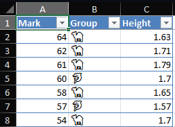
Let’s make our sheet look better

n <- 100
data.frame(
  Mark = rbinom(n, 100, 0.6), 
  Group = c('🐬', '🐪') |> sample(n, replace = TRUE), 
  Height = rnorm(n, 1.67, 0.1) |> round(2)
) |> openxlsx::write.xlsx(
        'gen_data_2.xlsx', 
        firstRow = TRUE, 
        asTable = TRUE,
        colWidths = c(10, 11, 12) # or "auto"
     )

You can go much fancier than this. The openxlsx and openxlsx2 packages allow for crazy customisation.

Multiple data sets

Excel workbooks can have many sheets, there is no need to write to different files each time.

Give every student their own data set

Students like to ‘work together’
- Unfortunately not in a good way
- Instead of collaborative learning, it often degenerates into one person doing all the work (and thus all the learning)
Partial solution: randomised assessment
I’ve been a driver of randomised assessment since 2006
- Started with WebCT (previous name for Blackboard) ‘Calculated’ questions.
R exams package makes it easy to generate a BB quiz with different numbers for every student
- Still automatic marking!

Cycling through students

We only need about 3 more lines of code 😊

students <- c('2024000001', '2024000002', '2024000003', '2024000004',
              '2024000005') # Get class list in R somehow
# You can read student numbers from class list / mark list file:
# students <- openxlsx::read.xlsx('mark_list.xlsx', startRow = 4)$Student.ID
n <- 100
students |> lapply(\(s) {   # Make a list of data frames
  data.frame(
    Mark = rbinom(n, 100, 0.6), 
    Group = c('🐬', '🐪') |> sample(n, replace = TRUE), 
    Height = rnorm(n, 1.67, 0.1) |> round(2)
  )
}) |> setNames(students) |> # Give the data frames names
  openxlsx::write.xlsx('gen_data_3.xlsx', 
        firstRow = TRUE, asTable = TRUE,
        colWidths = c(10, 11, 12) # or "auto"
     )

More interesting simulations

Students engage better with assignments that are relatable.

Steps for generating a realistic looking data set

Come up with a topic. A business problem, a scientific problem, or a social problem work best.
Think up some variables that would theoretically be practically measurable.
Generate latent variables and hyperparameters, such as number of observations, groups, underlying values, and residuals.
Generate the variables that depend on the above.
Give them nice names and save.

Variables should depend on each other

Real data is never truly i.i.d., but real data that fits the patterns we want to test is really tough to find
Easy compromise: conditional independence, i.e. regression
Try to have variables depend on other variables plus noise, not just noise

n <- 100
x1 <- runif(n, 20, 30) |> ceiling() # random integer from 21 to 30
x2 <- (x1*2 + 1 + rnorm(n)) |> round(2)
d <- data.frame(
  Age = x1,
  Spending = x2
)

Even more interesting simulations

What about time series? We could simulate a pair of \(VARIMA_2(1,1,1)-tGARCH(1,1)\) financial time series like so:

n <- 120
e <- mvtnorm::rmvt(n, sigma = c(1, 0.5, 0.5, 1) |> matrix(2), df = 4)
x1 <- x2 <- v1 <- v2 <- rep(1, n)
for (i in 2:n) {
  v1[i] <- 0.5 + 0.2*e[i-1, 1]^2 + 0.3*v1[i-1]
  v2[i] <- 0.5 + 0.2*e[i-1, 2]^2 + 0.3*v2[i-1]
  e[i,] <- e[i,] * sqrt(c(v1[i], v2[i]))
  x1[i] <- 0.1 + 0.3*x1[i-1] + 0.3*e[i-1, 1] + e[i, 1]
  x2[i] <- 0.12 + 0.35*x2[i-1] + 0.2*e[i-1, 2] + e[i, 2]
}
d <- data.frame(
  Month = seq_len(n-20), 
  ABC = cumsum(x1[21:n]/60) |> exp() + 30,
  DEF = cumsum(x2[21:n]/50) |> exp() + 29.5
)

Check your work

Before saving to Excel, do a plot or summary, or even a full analysis, in R. You might save yourself a lot of hassle in the long run.

Conclusion

Summary

We saw that generating good looking spreadsheets of data can come from a few lines of code.
A few more lines of code and anything is possible (within statistical reason).
Giving students different data sets slightly reduces copying.

This presentation was created using the Reveal.js format in Quarto, using the RStudio IDE. Font and line colours according to UFS branding, and background image using image editor GIMP by compositing images from CoPilot (DALL-E_v3).