Robust Bayesian statistical modelling for reliable inference and prediction with uncertainty
Sean van der Merwe
Introduction
Statistical regression modelling is used to relate one set of measurements to another set of measurements, or to predict a quantity based on observed quantities.
Abstract
Beginning with examples of statistical regression models fitted for the NAS faculty in recent years, the basic assumptions of standard statistical modelling are explained. Then the common measures of location (mean, median, mode) are discussed and illustrated. The presentation will dig into the relevance and uses of each, and then explain their role in parametric regression models. In particular, the connection or disconnection between the measure of location used in the model and the measure of location implied by the problem may help researchers avoid making misleading conclusions. Further, by first understanding and then changing the underlying assumptions of statistical models, one can obtain robust results that retain accurate predictive coverage. Examples will be drawn from a selection of recent papers focussing on robust mixed-effects regression models, including quantile regression models and joint modules. Robust here referring to models less influenced by outliers and skewness.
Keywords: regression; parametric model; skewness; robust regression; quantile regression
Measures of location
Where are your measurements situated on the number line?
Non-symmetry illustration
What would you consider to be the typical value for something like income? Is it any of these?
For the measurements you model, what is the explanatory structure actually related to?
Non-symmetric conditional distributions
- For symmetric distributions such as the normal, logistic, and t distributions:
- \(\mu\ \equiv\) mean \(\equiv\) median \(\equiv\) mode
- For the rest we have to explicitly state what we are trying to explain
When building models, ask yourself whether you are trying to model or predict, then ask yourself whether you are trying to model or predict
- The expected value (mean)
- The middle value (median)
- The most likely value (mode)
Log-transform example
- Suppose your values are very skew to the right (some values much larger than others) then it is common to take a log transform to avoid those extreme values dominating the analysis.
- OLS regression then assumes a conditional normal distribution
\[\begin{aligned} \log Y_i & \sim N\left(\mu_i = \mathbf{x}_i \boldsymbol\beta,\ \sigma^2\right) \\ \equiv Y_i & \sim logN\text{ with median }e^{\mu_i}=e^{\beta_0+\beta_1 x_{1i}+\dots} \end{aligned}\]
- On the original scale you’ve actually fitted a multiplicative model for the median.
- If done directly this would be called a non-linear quantile regression model.
Quantile regression
- We don’t have to focus only on the relationship between the explanatory variables and the expected or typical value!
- Have you ever considered regression on the 95% Value-at-Risk (VaR) directly?
- The factors explaining it might be quite different to the factors explaining the expected value.
The simplest quantile regression is median regression. One way to do it is to just replace the normal distribution with a Laplace distribution (double exponential - one exponential tail pointing left and one pointing right).
From the Laplace distribution the logical evolution is the Skew Laplace distribution. For this distribution the lower quantiles produce right skew and upper quantiles produce left skew. This makes sense when modelling a simple sample but it makes less sense when modelling residuals, where upper observations could easily have right skew residuals.
Instead, I would recommend the skew exponential power distribution for flexible modelling.
\[F_{\text{SEP}}\left(y \left| \mu, \sigma, \kappa_1, \kappa_2, p_0 \right.\right) = \begin{cases} p_0 \left(1 - G\left(\frac{1}{\kappa_1}\left(\frac{\mu - y}{2 p_0 \sigma K_1}\right)^{\kappa_1}, \frac{1}{\kappa_1}\right)\right), & y \leq \mu, \\ p_0 + \left(1 - p_0\right) G\left(\frac{1}{\kappa_2}\left(\frac{y - \mu}{2\left(1 - p_0\right) \sigma K_2}\right)^{\kappa_2}, \frac{1}{\kappa_2}\right), & y > \mu, \end{cases}\]
where \(G\left(a, b\right)\) is the regularized incomplete gamma function:
The SEP distribution reduces to a normal distribution with mean \(\mu\) and standard deviation \(\sigma/\sqrt{2\pi}\) when \(p_0 = 0.5\) and \(\kappa_1 = \kappa_2 = 2\). When \(p_0 = 0.5\) and \(\kappa_1 = \kappa_2 = 1\), it becomes the symmetric Laplace distribution. As \(\left(\kappa_1, \kappa_2\right) \to \infty\), the SEP distribution approaches a uniform distribution.
If we vary \(\kappa_2\) it changes the right shape independently of \(p_0\).
Curvy data
Sometime you just want to fit a curve, but even then …
Why distributions?
If you only care about predictions
then just use the most accurate model (depending on your data size and structure) and optimise it using your loss function of choice. Works well when you have a lot of data.
Note
In a linear model optimising with squared error loss is equivalent to maximising a normal distribution likelihood. The loss function is like a distribution and matters a lot.
But note that a point estimate is always wrong
One of the main things that drive statisticians is wanting to understand uncertainty.
Coverage
Which interval is more useful?
- Channel A says they’re 95% sure tomorrow’s maximum temperature is going to be between -20 and 46.
- Channel B says they’re 95% sure tomorrow’s maximum temperature is going to be between 20 and 26.
- Channel C says they’re 3% sure tomorrow’s maximum temperature is going to be 23 (i.e. between 22.5 and 23.5).
Shorter intervals carry more information than wider intervals, and intervals carry more information than point estimates, but only if they’re valid.
- A 95% interval should cover the target value 95% of the time.
Bayesian Inference
Inference is about going small to big
We perform experiments and collect samples because we want to understand the bigger picture - the data generating process.
The specific sample is often not important. For example, a pharmaceutical company is far more interested in future paying customers than the ones they paid to take part in their clinical trial.
- The biggest reason I like Bayesian parametric regression models is because they can do inference while still producing useful predictions with accurate coverage.
- They can accurately describe both the patterns and uncertainty for future data.
- Frequentist models focus on inference, while Data Science models (see also machine learning, big data, AI models, etc.) focus on predictions.
- I am convinced that the Bayesian models make inference easier and more reliable while still making useful predictions.
Inference example: river cleanup
Constructing a model that has a single parameter that captures the research question, yet also captures the variation, is very useful.
Here we want to know how much pollution was cleaned up each month, but much of the data was censored. It’s tricky to model the data when you don’t measure it exactly, but not impossible.
Example: HIV Viral Load
The ACTG 315 dataset, available in the ushr R package, includes longitudinal measurements of HIV viral load (log\(_{10}\) RNA copies/mL) over time. It features data on 46 patients, with the longest measurement recorded on Day 196 after baseline (Day 0).
Data set
RNA by time and subject
Quantile regression fits
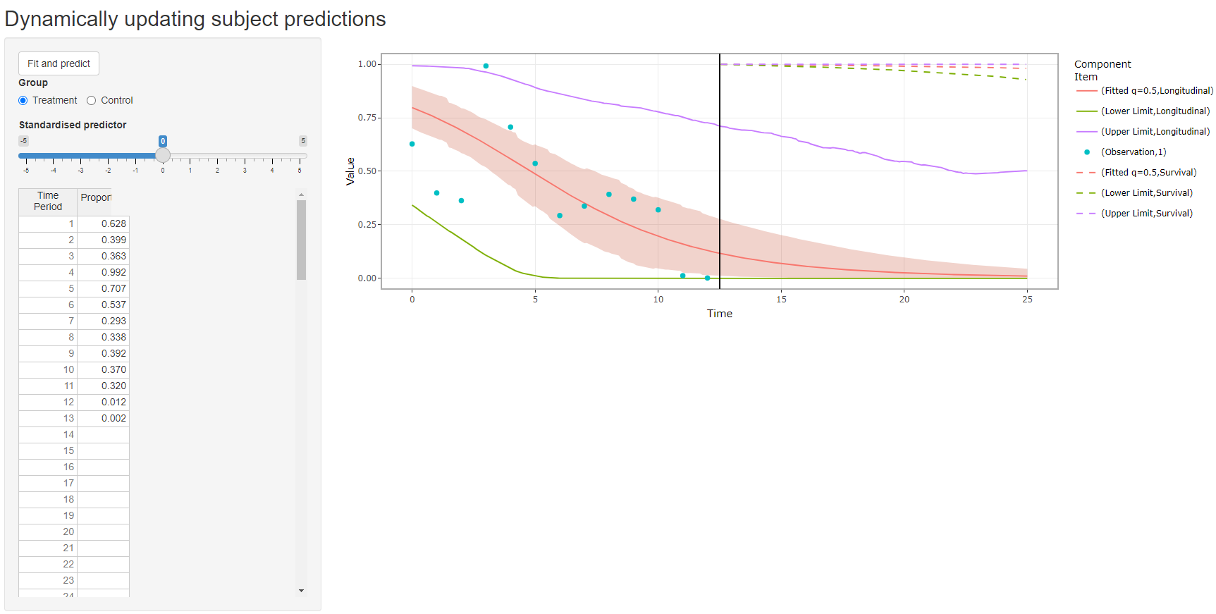
Example: Medication adherence
In this study you are interested in how long people are going to keep taking the medication (persistence) and how consistently they are taking the medication (adherence). Further, you know that these two behaviours interact, and you want to know what the effect of an intervention is on the joint behaviour.
In this case we fitted a joint model where the output of the adherence model feeds into the persistence model.
Adherence and persistence


Adherence by age, time, and treatment
Web interface
- The company that owns the data (typically the one who developed the medication) can host an app on their website that would allow a doctor or pharmacist to type in a patient’s record anonymously and get reasonable predictions.
Example: Giraffes
The giraffe video data
Kaitlyn Taylor, M student in Animal Science, went to 3 reserves and filmed 252 video of giraffes reacting to sounds that she played them, then coded the behaviours for 180s from the sound (for 55 behaviours).

Conclusion
- An expansive statistical toolbox is incredibly useful when encountering real data.
- Real data is difficult but rewarding to work with.
- So expand your statistical toolbox to expand your impact.
This presentation was created using the Reveal.js format in Quarto, using the RStudio IDE. Font and line colours according to UFS branding, and background image using image editor GIMP by compositing images from CoPilot.

2026/06/24 - NAS Conference